library(tidyverse)
library(gtsummary)
library(dfmtbx)Linear Mixed-Effect Regression Models: Continuous Outcomes
Dataset description
The following tutorial is based on chapters 4 and 5 from Donald Hedeker and Robert Gibbons’ textbook “Longitudinal Analysis” and focuses on specifying mixed effect regression models in R and their interpretation using helper functions from the broom.mixed and gt_summary packages.
The example dataset comes from a 1977 study conducted by Reisby et. al on the effects of a tricyclic anti-depressant drug, imipramine, on clinical ratings of depression and its metabolites, (imipramine and desipramine). Tri-cyclic antidepressants are a class of drugs that were more commonly used before the development of the newer anti-depressants like selective-serotonin-reuptake-inhibitors (SSRIs) and selective-norepinephrine-reuptake-inhibitors (SNRIs). Following a 1 week placebo period, 66 hospitalized patients were treated with a 225 mg/day dose of imipramine for 4 weeks.
The first dataset can be obtained from Don Hedeker’s Statistical Site and contains three variables. First, the “time” variable, weeks 0 through 6, where week 0 represents a baseline time point and week 1 represents the placebo period. Weeks 2 through 6 represent the time periods where the drug was administerd. Next, the primary outcome is a depression score (hamd), from the Hamilton Rating Scale (HRS). Although multiple versions of this scale exist, we will suppose that the data utilize the 17-item version. In this version, 0-7 would indicate normal (no depression), 8-13 would indicate mild depression, 14-18 would indicate moderate depression, 19-22 is severe depression, and anything over 22 is very severe. Finally, a time-invariant covariate (endogenous), describes whether the patient’s depression was precipitated by an external event such as the death of a loved one (non-endogenous) or developed spontaneously (endogenous).
In a subsequent dataset consisting of weeks 2 through 6, plasma levels of imipramine and its metabolite, desipramine, are available as time-varying covariates from the multilevelmod package.
Exploratory data analysis
# Prepare data by converting to tibble and setting subject as factor
data <- data %>%
  as_tibble() %>%
mutate(subject = factor(subject))str(data)tibble [396 × 4] (S3: tbl_df/tbl/data.frame)
$ subject : Factor w/ 66 levels "101","103","104",..: 1 1 1 1 1 1 2 2 2 2 ...
$ week : num [1:396] 0 1 2 3 4 5 0 1 2 3 ...
$ hamd : num [1:396] 26 22 18 7 4 3 33 24 15 24 ...
$ endogenous: num [1:396] 0 0 0 0 0 0 0 0 0 0 ...# Display the first 6 rows of data
data %>%
head() %>%
style_gt_tbl()| subject | week | hamd | endogenous |
|---|---|---|---|
| 101 | 0 | 26 | 0 |
| 101 | 1 | 22 | 0 |
| 101 | 2 | 18 | 0 |
| 101 | 3 | 7 | 0 |
| 101 | 4 | 4 | 0 |
| 101 | 5 | 3 | 0 |
Generate summary statistics
# source("C:\\Users\\rodrica2\\OneDrive\\Web Site\\quarto_website\\personal-site\\functions\\summarize_column.R")

summary_stats <- data %>%
  group_by(week) %>%
  summarize_variable(., hamd)
summary_stats %>%
format_gt_tbl()| week | n | min | max | median | mean | sd | se |
|---|---|---|---|---|---|---|---|
| 0 | 61 | 15 | 34 | 22 | 23.44 | 4.53 | 0.580 |
| 1 | 63 | 11 | 39 | 22 | 21.84 | 4.70 | 0.592 |
| 2 | 65 | 10 | 33 | 18 | 18.31 | 5.49 | 0.680 |
| 3 | 65 | 0 | 32 | 16 | 16.42 | 6.42 | 0.796 |
| 4 | 63 | 0 | 34 | 12 | 13.62 | 6.97 | 0.878 |
| 5 | 58 | 0 | 33 | 11 | 11.95 | 7.22 | 0.948 |
After inspecting the means by week we notice a few characteristics. First, it appears as though mean hamd scores decrease over time. If we interpret these means based on the 17-item version of the HRS, the average hamd score at week 0 falls in the very severe range of depression. By the end of the study, the average scores improves and falls in to the mild depression range.
Next, the standard deviations of mean depression ratings increase over time which suggest increasing levels of variability.
Finally, although 66 subjects were enrolled in the study, the number of data points per week is not constant. This indicates that there are missing values in the dataset and part of the reason why a linear mixed effect regression model is implemented. In order to analyze these data with a univariate repeated measures ANOVA or a multivariate ANOVA, we would have to drop data from 20 subjects, which would represent approximately 30% of the sample and might bias our results.
data %>%
  drop_na() %>%
  group_by(subject) %>%
  count() %>%
  ungroup() %>%
  filter(n == 6) %>%
  summarise(n_complete = n_distinct(subject)) %>%
style_gt_tbl()| n_complete |
|---|
| 46 |
Inspect correlations
After inspecting the summary statistics, it may be good idea to inspect the correlation of the outcome at one time point to another. This step can help us better understand temporal patterns in the data. For example, high correlations between time points could signal that a variable is consistent and displays trait-like properties. On the other hand, low correlations could signal that a variable displays state-like variability. Another reason to inspect correlations is to better incorporate the covariance structure into a model that can improve model fit, reduce bias, and lead to better inferences.
Before calculating the correlations, we need to structure our data into wide format.
cor_data_wide <- data %>%
  pivot_wider(names_from = week, values_from = hamd) %>%
  select(-endogenous, -subject)
cor_data_wide %>%
head() %>%
style_gt_tbl()| 0 | 1 | 2 | 3 | 4 | 5 |
|---|---|---|---|---|---|
| 26 | 22 | 18 | 7 | 4 | 3 |
| 33 | 24 | 15 | 24 | 15 | 13 |
| 29 | 22 | 18 | 13 | 19 | 0 |
| 22 | 12 | 16 | 16 | 13 | 9 |
| 21 | 25 | 23 | 18 | 20 | NA |
| 21 | 21 | 16 | 19 | NA | 6 |
There are two possible approaches to calculating and displaying correlations. In the first approach, we use the “complete.obs” option in the cor() function. This performs listwise deletion which is the same as dropping any row that contains at least one missing value. In this approach, the number of data points used for each pairwise correlation is the same.
cor_data_wide %>%
  cor(., use = "complete.obs") %>%
  as_tibble() %>%
  round(2) %>%
  mutate(week = c(0:5)) %>%
  select(week, everything()) %>%
style_gt_tbl()| week | 0 | 1 | 2 | 3 | 4 | 5 |
|---|---|---|---|---|---|---|
| 0 | 1.00 | 0.49 | 0.42 | 0.44 | 0.30 | 0.22 |
| 1 | 0.49 | 1.00 | 0.49 | 0.51 | 0.35 | 0.23 |
| 2 | 0.42 | 0.49 | 1.00 | 0.73 | 0.68 | 0.53 |
| 3 | 0.44 | 0.51 | 0.73 | 1.00 | 0.78 | 0.62 |
| 4 | 0.30 | 0.35 | 0.68 | 0.78 | 1.00 | 0.72 |
| 5 | 0.22 | 0.23 | 0.53 | 0.62 | 0.72 | 1.00 |
In the second approach, we use the “pairwise.complete.obs” option in the cor() function. This option tells R to examine each pair of time points individually and then drop any rows with a missing value. This approach is also called pairwise deletion and can result in each pairwise correlation having a different number of data points.
# Correlations of the observations
# pairwise.complete.obs excludes values from subjects in a pairwise fashion.
# Each correlation will not have the same n. Values are excluded by only
# considering the two timepoints for each correlation
cor_data_wide %>%
  cor(., use = "pairwise.complete.obs") %>%
  as_tibble() %>%
  round(2) %>%
  mutate(week = c(0:5)) %>%
  select(week, everything()) %>%
style_gt_tbl()| week | 0 | 1 | 2 | 3 | 4 | 5 |
|---|---|---|---|---|---|---|
| 0 | 1.00 | 0.49 | 0.41 | 0.33 | 0.23 | 0.18 |
| 1 | 0.49 | 1.00 | 0.49 | 0.41 | 0.31 | 0.22 |
| 2 | 0.41 | 0.49 | 1.00 | 0.74 | 0.67 | 0.46 |
| 3 | 0.33 | 0.41 | 0.74 | 1.00 | 0.82 | 0.57 |
| 4 | 0.23 | 0.31 | 0.67 | 0.82 | 1.00 | 0.65 |
| 5 | 0.18 | 0.22 | 0.46 | 0.57 | 0.65 | 1.00 |
Visualize data
To visualize the data, we can employ the ggplot2 package and the long format data frame. First we drop the missing values, specify the x and y variables in the aes() function, and then specify that we want our data to be grouped and colored by subject. Next, we can use the line() and point() geoms to draw lines with points at each week. Since there are 66 subjects, there will be 66 colors added to the legend which can be removed with the legend.position = “none” option.
# Visualize each subjects trend
data %>%
  drop_na(hamd) %>%
  ggplot(., aes(x = week, y = hamd, group = subject, color = subject)) +
  geom_line() +
  geom_point() +
  theme_minimal() +
  theme(legend.position = "none")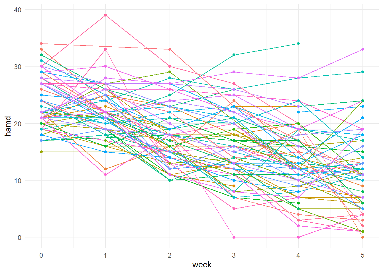
Random intercept model
Perhaps the most basic mixed effect regression model is the random intercept model which can be viewed as an extension of an ordinary least squares model (OLS). In the OLS framework, a single intercept and a single slope is estimated. In contrast, the random intercept model allows each subject to have their own intercept, effectively giving each individual a unique baseline or starting point. However, both OLS and random intercept models assume a common slope or rate of change across subjects.
In this example, time is modeled as a continuous variable. If time were modeled as a discrete factor instead and the data contained no missing values, the random intercept model would closely resemble the results of a univariate repeated measures ANOVA.
# HAMD scores modeled as a function of week with subject-specific intercepts to
# capture individual differences at baseline. Hedeker & Gibbons fit these data
# with Maximum Likelihood (ML) estimation which is specified with the REML =
# FALSE option. REML is the default in the lmer() function. In subsequent
# steps, ML estimation will help with model comparisons via the Likelihood
# Ratio Test (LRT).
model_tab_4.3 <- lmerTest::lmer(
  hamd ~ week + (1 | subject),
  data = data,
  REML = FALSE
)
Output
After fitting a model using the lmer() function, there are several ways to display the results. The most comprehensive is the base R summary() function, which provides a wealth of information that includes fit diagnostics, parameter estimates for both fixed and random effects, and p-values (if the lmerTest package is used).
summary(model_tab_4.3)Linear mixed model fit by maximum likelihood . t-tests use Satterthwaite's
method [lmerModLmerTest]
Formula: hamd ~ week + (1 | subject)
Data: data
AIC BIC logLik -2*log(L) df.resid
2293.2 2308.9 -1142.6 2285.2 371
Scaled residuals:
Min 1Q Median 3Q Max
-3.1739 -0.5876 -0.0342 0.5465 3.5297
Random effects:
Groups Name Variance Std.Dev.
subject (Intercept) 16.16 4.019
Residual 19.04 4.363
Number of obs: 375, groups: subject, 66
Fixed effects:
Estimate Std. Error df t value Pr(>|t|)
(Intercept) 23.5518 0.6385 121.3320 36.88 <2e-16 ***
week -2.3757 0.1350 310.9879 -17.60 <2e-16 ***
---
Signif. codes: 0 '***' 0.001 '**' 0.01 '*' 0.05 '.' 0.1 ' ' 1
Correlation of Fixed Effects:
(Intr)
week -0.524One drawback, however, is that the output from summary() is not easily formatted into tables that render cleanly in .html or .docx documents generated from a Quarto .qmd file. Personally, I prefer using .qmd files for output because they produce visually digestible results, are easy to share with colleagues, and facilitates copy-pasting output into other formats like .xlsx.
A second approach to displaying model output is to use the tbl_regression() function from the gtsummary package. This function creates a clean, publication-ready table of regression results and can be paired with add_glance_table() to include additional model fit statistics. Together, they produce a well-formatted table that renders seamlessly in .html or .docx outputs from a Quarto .qmd document.
tbl_regression(model_tab_4.3,
               intercept = TRUE,
               estimate_fun = purrr::partial(style_ratio, digits = 4)) %>%
add_glance_table(include = c("nobs", "sigma", "logLik", "AIC", "BIC", "df.residual"))| Characteristic | Beta | 95% CI | p-value |
|---|---|---|---|
| (Intercept) | 23.552 | 22.288, 24.816 | <0.001 |
| week | -2.3757 | -2.6412, -2.1101 | <0.001 |
| No. Obs. | 375 | ||
| Sigma | 4.36 | ||
| Log-likelihood | -1,143 | ||
| AIC | 2,293 | ||
| BIC | 2,309 | ||
| Residual df | 371 | ||
| Abbreviation: CI = Confidence Interval | |||
The main drawback of this approach is that it omits much of the granular detail provided by the summary() function—such as random effect estimates, residual diagnostics, and full variance-covariance information.
A third approach to summarizing model output is to use the tidy() function from the broom.mixed package. On its own, tidy() returns a tibble containing estimates for both fixed and random effects. It also includes the standard deviations of random effects and residuals, which can be useful for assessing model fit. In addition, the glance() function from the same package, displays information such as the number of observations, the Akaike Information Criterion (AIC), the Bayesian Information Criterion (BIC), and the deviance which is equal to -2 * the log likelihood (logLik).
This approach closely resembles the format used by Hedeker and Gibbons in their text. The main difference is that tidy() displays standard deviations instead of variances and correlations instead of covariances. This format is used for displaying the remaining models in the tutorial.
One advantage of returning a tibble is that it can be piped into the gt() function to produce a well-formatted table that renders cleanly in .html or .docx outputs from a Quarto .qmd file. In this case, I’ve piped the tidy() output into a custom function that formats the tibble into a gt table with bolded headings and formatted p-values.
broom.mixed::tidy(model_tab_4.3) %>%
format_gt_tbl()| effect | group | term | estimate | std.error | statistic | df | p.value |
|---|---|---|---|---|---|---|---|
| fixed | (Intercept) | 23.55 | 0.639 | 36.88 | 121.33 | < 0.001 | |
| fixed | week | −2.38 | 0.135 | −17.60 | 310.99 | < 0.001 | |
| ran_pars | subject | sd__(Intercept) | 4.02 | ||||
| ran_pars | Residual | sd__Observation | 4.36 |
broom.mixed::glance(model_tab_4.3) %>%
format_gt_tbl()| nobs | sigma | logLik | AIC | BIC | deviance | df.residual |
|---|---|---|---|---|---|---|
| 375 | 4.36 | −1,142.59 | 2,293.19 | 2,308.90 | 2,285.19 | 371 |
Interpretation
The 4 rows of the tidy() model output can be interpreted as follows:
- the fixed effect (Intercept) is the estimated hamd score at week 0. This effect is statistically significant (p < 0.001), indicaing that it differs from zero. However, its interpretive value is limited, as it primarily serves as a baseline reference.
- The fixed effect of week suggests that on average, patients experience a 2.38-point reduction in hamd scores for each additional week in the study. This effect is statistically significantly and supports the conclusion that imipramine reduces depression symptoms over time.
- The random effect sd__(Intercept), 4.02, reflects the estimated standard deviation of subject-specific intercepts in the population centered on a mean of 23.6. This captures variability in baseline depression levels across individuals. As an important note, the population in question consists of patients hospitalized for depression and not necessarily the general population.
- The sd__Observation is the standard deviation of the residuals, representing the average deviation between observed and predicted hamd scores. It reflects within-subject variability not explained by the model. This value is labelled as sigma in the tbl_regression() and glance() table outputs.
Compare estimated means
emmeans::emm_options(lmer.df = "satterthwaite")

emmeans_week <- emmeans::emmeans(
  model_tab_4.3, ~ week,
  at = list(week = c(0, 1, 2, 3, 4, 5)))
# Compare the observed and predicted means to gauge model fit
summary_stats %>%
select(week, mean) %>%
left_join(
emmeans_week %>% as_tibble() %>% select(week, emmean),
by = "week") %>%
format_gt_tbl()| week | mean | emmean |
|---|---|---|
| 0 | 23.44 | 23.55 |
| 1 | 21.84 | 21.18 |
| 2 | 18.31 | 18.80 |
| 3 | 16.42 | 16.42 |
| 4 | 13.62 | 14.05 |
| 5 | 11.95 | 11.67 |
ICC
# Calculate the ICC, by extracting the covariance parameter estimates from the
# model summary output in element number 13, then squaring. The first row
# corresponds to the subject and the second row corresponds to the residual.
# The variable var will thus contain the subject and residual variances as a
# vector.
cov_parameter_estimates <-
  summary(model_tab_4.3)[[13]] %>%
  as.data.frame() %>%
  select(sdcor) %>%
  mutate(var = sdcor^2)

# icc = cov_subj / cov_subj + cov_residual
icc <- cov_parameter_estimates$var[1] / sum(cov_parameter_estimates$var)

icc %>%
  as_tibble() %>%
  round(2) %>%
style_gt_tbl()| value |
|---|
| 0.46 |
An ICC of 0.46 indicates that 46% of the total variance in hamd scores is attributable to differences between subjects, and 54% is attributable to within-subject variation across time. A higher ICC suggests subjects are more consistent within themselves and more different from each other. A lower ICC suggests more variability within subjects across time relative to between-subject differences.
OLS Model
Fitting the same data to an OLS simple linear regression model that ignores the clustering of data points within individuals, yields results that are in close agreement with the random-intercept model. However the SEs are different because the error variance is lumped together in the OLS model as opposed to partitioned out into between and within subject variances in the mixed model.
ols_model <-
  lm(hamd ~ week, data = data)

broom::tidy(ols_model) %>%
format_gt_tbl()| term | estimate | std.error | statistic | p.value |
|---|---|---|---|---|
| (Intercept) | 23.60 | 0.548 | 43.10 | < 0.001 |
| week | −2.41 | 0.183 | −13.16 | < 0.001 |
Random intercept and slope model
Building off of the previous mixed effect model, we now add a random slope for week. This allows each subject to have their own rate of change in addition to their own baseline (intercept). This means that the model accounts for individual differences not only where subjects start, but also how they progress over time. This allows for more flexible and realistic modeling of longitudinal data where individuals may respond differently over time.
# HAMD scores modeled as a function of week with subject-specific intercepts
# and slopes to capture individual differences in baseline and rates of change.
model_tab_4.5 <- lmerTest::lmer(
  hamd ~ week + (1 + week | subject),
  data = data,
  REML = FALSE
)

# Adding the conf.int = TRUE option displays 90% confidence intervals for the
# fixed effects.
broom.mixed::tidy(model_tab_4.5, conf.int = TRUE) %>%
format_gt_tbl()| effect | group | term | estimate | std.error | statistic | df | p.value | conf.low | conf.high |
|---|---|---|---|---|---|---|---|---|---|
| fixed | (Intercept) | 23.58 | 0.546 | 43.22 | 63.76 | < 0.001 | 22.49 | 24.67 | |
| fixed | week | −2.38 | 0.209 | −11.39 | 63.10 | < 0.001 | −2.79 | −1.96 | |
| ran_pars | subject | sd__(Intercept) | 3.55 | ||||||
| ran_pars | subject | cor__(Intercept).week | −0.28 | ||||||
| ran_pars | subject | sd__week | 1.44 | ||||||
| ran_pars | Residual | sd__Observation | 3.50 |
Interpretation
- The fixed effect for (Intercept) tells us that on average, the predicted hamd score at week 0 is 23.6 points. One way to illustrate this is to use the augment() function from the broom.mixed package to get the predicted values, filter the rows where week == 0 only and then average them. The result equals the (Intercept) in the output.
broom.mixed::augment(model_tab_4.5) %>%
  filter(week == 0) %>%
summarise(mean_predicted_vals = mean(.fitted))- The fixed effect of week tells us that for every 1 unit increase in week, we can expect a drop of 2.38 points. In other words, on average, patients drop 2.38 points in hamd scores each week. This is a significant effect which indicates that hamd scores decrease over time.
- The sd_(Intercept) is the estimate of the standard deviation of a distribution of intercepts centered on 23.58.
- -0.28 is the correlation between the intercept and the slope. It tells us that subjects who are more depressed at baseline tend to have a steeper rate of change. In these data, however, it could also be viewed as a floor effect because those with lower initial scores, who are less depressed, have less room to improve.
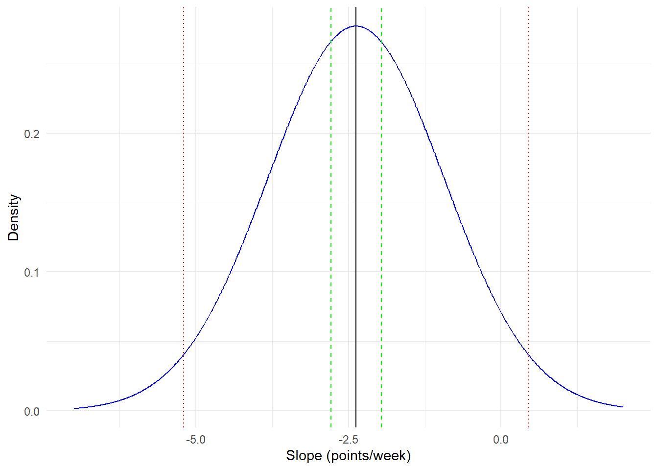
- The sd_week, 1.44, is an estimate of the population standard deviation for the parameter estimate of the fixed effect for week. An interval using the sd__week in row 5 can be constructed as -2.38 +/- (1.96 * 1.44) = -5.20 to 0.44. This interval reflects the distribution of individual rates of change around the average slope (week). In this case, it tells us that while the average rate of change is negative, the spread of the distribution of slopes is large enough to include 0 (no change) and some slightly positive slopes. In other words, most people tend to improve, but some may not, and others still may get slightly worse.
It is important to distinguish between the confidence interval given in row 2 for the fixed effect of week and the interval constructed using the sd__week in row 5 in Model table 4.5. The estimate in row 2 tells us that the average rate of change is a drop of -2.38 points for each week the subject is in the study. The corresponding confidence interval tells us that we are 95% confident that the true rate of change in the population lies between -2.79 and -1.96. The interval constructed using sd__week is more about the spread of the distribution of slopes centered on the average slope for week (-2.38).
- The sd of the residuals. This is the within-subject variability not explained by the fixed or random effects. A large sd here would mean that the data is noisy, and a small sd would indicate the model fits the data well. The size of sd is relative to the outcome. 3.5 out of 52 (max hamd score) is 6.7% of the scale indicating some but not severe level of residual variation.
Visual demonstration of intervals
Likelihood ratio test
The likelihood ratio test (LRT) is one way to determine if adding an additional term to the model improves the fit significantly. We can conduct a LRT between the model with the random intercept and the model with the random intercept AND random slope since the former can be considered as nested within the latter. To do this we can use the anova() function specifying the two models as inputs and examining the chi-square statistic.
broom::tidy(anova(model_tab_4.3, model_tab_4.5)) %>%
format_gt_tbl()| term | npar | AIC | BIC | logLik | minus2logL | statistic | df | p.value |
|---|---|---|---|---|---|---|---|---|
| model_tab_4.3 | 4 | 2,293.19 | 2,308.90 | −1,142.59 | 2,285.19 | |||
| model_tab_4.5 | 6 | 2,231.04 | 2,254.60 | −1,109.52 | 2,219.04 | 66.15 | 2 | < 0.001 |
The result of the LRT is statistically significant (p < 0.001), which indicates that adding the random effect for individual slopes improves the model fit. This means that allowing each subject to have their own rate of change explains meaningful variability in the data. If each subject has their own rate of change, then it follows that compound symmetry is rejected. This is because compound symmetry implies a constant rate of change for each subject.
In compound symmetry, we assume two properties of the data. First, the variances of the outcome at each timepoint are equal. Second, we also assume that the covariances between any two time points are the same. These conditions are met only if each subject has the same rate of change, although each subject can have a different baseline.
Part of the rationale for mentioning this is because one of the assumptions of the univariate repeated measures ANOVA is sphericity. Although sphericity is the technical assumption, it is rarely met in practice unless compound symmetry is also met. As mentioned earlier, the assumption of compoound symmetry implies the same rate of change for each subject. This may be too restrictive of an assumption and mixed effect regression models help overcome this shortcoming.
Coding of time
Time can be coded in a different ways in a mixed effect regression model. Here the middle of the study is set to 0. Thus the interpretation of the intercept changes to reflect the predicted value when time (week) = 2.5. The intercept will differ from the previous model with a random intercept and random slope, but the fixed effect of week will be the exact same. In a similar vein, because the intercept has changed, the variance of the (Intercept) will be different than the random intercept and slope model. We also see that the correlation between the intercept and slope is now positive. This indicates that higher mid-study depression is associated with positive slopes. Another way to interpret this is that those that have higher depression scores mid study have less negative or more positive slopes, as if they are not responding to the medication with the same intensity in the earlier weeks.
data <- data %>%
  mutate(weekc = week - 2.5)

# HAMD scores modeled as a function of week centered at 2.5 with subject
# specific intercepts and slopes to capture individual differences in
# baseline and rates of change.
model_tab_4.6 <- lmerTest::lmer(
    hamd ~ weekc  + (1 + weekc | subject),
    data = data,
    REML = FALSE)

broom.mixed::tidy(model_tab_4.6) %>%
format_gt_tbl()| effect | group | term | estimate | std.error | statistic | df | p.value |
|---|---|---|---|---|---|---|---|
| fixed | (Intercept) | 17.63 | 0.560 | 31.47 | 65.74 | < 0.001 | |
| fixed | weekc | −2.38 | 0.209 | −11.39 | 63.11 | < 0.001 | |
| ran_pars | subject | sd__(Intercept) | 4.30 | ||||
| ran_pars | subject | cor__(Intercept).weekc | 0.61 | ||||
| ran_pars | subject | sd__weekc | 1.44 | ||||
| ran_pars | Residual | sd__Observation | 3.50 |
Model with time-invariant covariate
One of the covariates in the example dataset describes whether or not the depresion was precipitated by an external event such as the death of a loved one (non-endogenous) or arose spontaneously (endogenous).
data %>%
  select(-weekc) %>%
  group_by(endogenous) %>%
  pivot_wider(names_from = week, values_from = hamd) %>%
  select(-subject) %>%
  mutate(endogenous = ifelse(endogenous == 1, "endogenous", "non-endogenous")) %>%
  tbl_summary(
    by = endogenous,
    statistic = list(everything() ~ "{mean}; {N_nonmiss}"),
    missing = "no",
    digits = list(everything() ~ 2)
  ) %>%
modify_header(label = "**week**")| week | endogenous N = 371 |
non-endogenous N = 291 |
|---|---|---|
| 0 | 24.00; 33.00 | 22.79; 28.00 |
| 1 | 23.00; 34.00 | 20.48; 29.00 |
| 2 | 19.30; 37.00 | 17.00; 28.00 |
| 3 | 17.28; 36.00 | 15.34; 29.00 |
| 4 | 14.47; 34.00 | 12.62; 29.00 |
| 5 | 12.58; 31.00 | 11.22; 27.00 |
| 1 Mean; N Non-missing | ||
# HAMD scores modeled as a function of the interaction between week and
# depression type (endogenous) allowing subject specific intercepts and slopes
# to capture individual differences in baseline and rates of change over time.
model_tab_4.8 <- lmerTest::lmer(
    hamd ~ week * endogenous + (1 + week | subject),
    data = data,
    REML = FALSE
)

broom.mixed::tidy(model_tab_4.8) %>%
format_gt_tbl()| effect | group | term | estimate | std.error | statistic | df | p.value |
|---|---|---|---|---|---|---|---|
| fixed | (Intercept) | 22.48 | 0.79 | 28.30 | 61.60 | < 0.001 | |
| fixed | week | −2.37 | 0.31 | −7.59 | 61.02 | < 0.001 | |
| fixed | endogenous | 1.99 | 1.07 | 1.86 | 63.21 | 0.068 | |
| fixed | week:endogenous | −0.03 | 0.42 | −0.06 | 62.70 | 0.949 | |
| ran_pars | subject | sd__(Intercept) | 3.41 | ||||
| ran_pars | subject | cor__(Intercept).week | −0.29 | ||||
| ran_pars | subject | sd__week | 1.44 | ||||
| ran_pars | Residual | sd__Observation | 3.50 |
- The fixed effect for (Intercept) tells us that on average, the predicted hamd score at week 0 for the non-endogenous group is 22.5 points.
- The fixed effect for week indicates that on average, we can expect a drop in 2.37 points in hamd scores for each additional week in non-endongenous subjects.
- The fixed effect for endogenous, tells us that on average, we can expect endogenous subjects to score 1.99 points higher than non-endogenous subjects. Furthermore, this effect is not significant which suggests that both groups have equal levels of depression.
- The fixed effect for week:endogenous represents the interaction between week and endogenous. It tells us that the effect of week is on average 0.03 points lower in the endogenous group compared to the non-endogenous group. In other words the rate of change in the endogenous group is slightly more pronounced. An additional, yet valid, interpretation, is the difference in slopes of endogenous and non-endogenous patients. However, the interaction is not significant which indicates this effect could be due to chance as opposed to the effect of the drug having a differential effect on the type of depression the subject has.
- The sd_(Intercept) is the estimated standard deviation of a distribution of intercepts from the population centered on 22.48.
- cor__(Intercept).week is the correlation between the baseline score and the effect of week. The value -0.29 which indicates that higher baseline scores are associated with steeper rates of change.
- sd__week is the estimated standard deviation of a distribution of slopes from the population centered on -2.37.
- sd__Observation is the standard deviation of the residuals
Likelihood ratio test
broom::tidy(anova(model_tab_4.5, model_tab_4.8)) %>%
format_gt_tbl()| term | npar | AIC | BIC | logLik | minus2logL | statistic | df | p.value |
|---|---|---|---|---|---|---|---|---|
| model_tab_4.5 | 6 | 2,231.04 | 2,254.60 | −1,109.52 | 2,219.04 | |||
| model_tab_4.8 | 8 | 2,230.93 | 2,262.34 | −1,107.46 | 2,214.93 | 4.11 | 2 | 0.128 |
The chi-square value 4.11 on 2 degrees of freedom and is not significant, indicating that the addition of the interaction term with depression type does not improve the model fit. As a result, the random intercept and random slope model is an adequate and more parsimonious model.
Model with time-varying covariates
For this portion of the chapter Hedeker and Gibbons use a subset of the data that consist of weeks 2 through 5, since these are the weeks when IMI and DMI covariates were collected. The data with the IMI and DMI variables are found in the multilevel mod package. In these data, week 0 represents week 2 of the study. The outcome, depression score, is represented as the change from baseline. The covariates are also log transformed to prevent the influence from extreme values since the raw data for imipramine range from 4 to 312 micrograms per liter for imipramine, and from 1 to 740 micrograms per liter for desipramine. This dataset will also need to be modified in two ways before fitting a model. First we need to merge the raw hamd scores into the data set. Second, we need to center the imipramine and desipramine variables.
# Create the data promise
data("riesby", package = "multilevelmod")

# Create and merge data
reisby <- riesby %>%
  # Merge the raw scores, by creating a week variable that is centered on week
  # 2 and are filtered for observations on or after the new week 0.
  left_join(data %>%
              mutate(week = week - 2) %>%
              filter(week >= 0) %>%
              select(subject, week, hamd),
            by = c("subject", "week")
            ) %>%
  # Center the covariates on their respective means
  mutate(I = imipramine - mean(imipramine),
         D = desipramine - mean(desipramine)) %>%
  # Rename the depr_score for clarity and brevity
  rename(delta = depr_score)
# HAMD scores modeled as a function of week, imipramine, and desipramine, with
# subject-specific intercepts and slopes for week to capture individual
# differences in baseline and rate of change.
model_tab_4.9 <- lmerTest::lmer(
hamd ~ week + I + D + (1 + week | subject),
data = reisby,
REML = FALSE
)
broom.mixed::tidy(model_tab_4.9) %>%
format_gt_tbl()| effect | group | term | estimate | std.error | statistic | df | p.value |
|---|---|---|---|---|---|---|---|
| fixed | (Intercept) | 18.17 | 0.707 | 25.70 | 65.40 | < 0.001 | |
| fixed | week | −2.03 | 0.284 | −7.15 | 66.33 | < 0.001 | |
| fixed | I | 0.60 | 0.850 | 0.71 | 131.01 | 0.480 | |
| fixed | D | −1.20 | 0.628 | −1.90 | 139.62 | 0.059 | |
| ran_pars | subject | sd__(Intercept) | 4.98 | ||||
| ran_pars | subject | cor__(Intercept).week | −0.09 | ||||
| ran_pars | subject | sd__week | 1.65 | ||||
| ran_pars | Residual | sd__Observation | 3.23 |
Interpretation
- The fixed effect for the (Intercept) 18.2 means that the predicted hamd score at study_week 2 for a patient with an average level of imiprimine and desiprimine is 18.2
- The fixed effect for week (-2.03) means that on average, we can expect a drop of 2.03 points in hamd scores for every additional week in the study. This effect is significant which indicates that patients improve in their depression over time.
- The fixed effect for the mean centered log Imiprimine is 0.602 and is not significant. Which means that mean centered log imiprimine is not a significant predictor of hamd scores.
- The fixed effect for the mean centered log Desiprimine is -1.20 and is not significant, which mean that the mean centered log desiprimine is not a significant predictor of hamd scores.
- The sd__(Intercept) is 4.98 and represents the estimated standard deviation of a distribution of population intercepts.
- The cor__(Intercept).week is -0.09 and indicates that the higher the hamd score at study_week 2, the lower the rate of change, but this is a very small correlation.
- The sd__week is the estimted standard deviation of a distribution of individual subject’s slopes from the population centered on the fixed effect of -2.03.
- The sd__observation is the standard deviation of the residuals.
Modeling the difference scores (delta) as the outcome
# HAMD change scores relative to baseline modeled as a function of week,
# imipramine, and desipramine, with subject-specific intercepts and slopes for
# week to capture individual differences in baseline and rate of change.
model_tab_4.10 <- lmerTest::lmer(
  delta ~ week + I + D + (1 + week | subject),
  data = reisby,
  REML = FALSE
)

broom.mixed::tidy(model_tab_4.10) %>%
format_gt_tbl()| effect | group | term | estimate | std.error | statistic | df | p.value |
|---|---|---|---|---|---|---|---|
| fixed | (Intercept) | −5.18 | 0.659 | −7.87 | 63.97 | < 0.001 | |
| fixed | week | −1.97 | 0.285 | −6.90 | 65.24 | < 0.001 | |
| fixed | I | 0.63 | 0.821 | 0.77 | 120.83 | 0.444 | |
| fixed | D | −1.97 | 0.602 | −3.26 | 128.05 | 0.001 | |
| ran_pars | subject | sd__(Intercept) | 4.53 | ||||
| ran_pars | subject | cor__(Intercept).week | 0.11 | ||||
| ran_pars | subject | sd__week | 1.67 | ||||
| ran_pars | Residual | sd__Observation | 3.24 |
Interpretation
- The fixed effect for the (Intercept), -5.18, refelects the predicted change score at study_week 2 for a patient with average levels of imiprimine and desiprimine.
- The fixed effect for week (-1.97) indicates that on average, we can expect a drop of 1.97 points in change scores for every additional week in the study.
- The fixed effect for the mean-centered log Imiprimine is 0.63. an is not statistically significant, but reflects the association between I and the change scores when holding all other variables constant.
- The fixed effect for the mean-centered log Desiprimine is -1.97 and is statistically significant. There is a negative association between mean-centered log desiprimine levels and change scores. For every unit increase in D, we can expect a 1.97 unit decrease in the change scores when holding all other variables constant.
- The sd__(Intercept), 4.53, reflects the estimated standard deviation of a distribution of intercepts in the population.
- The cor__(Intercept).week is -.11 and indicates that the higher the change score at study_week 2, the higher the rate of change. In other words, the rate of change tends to be higher in those with higher change scores at study_week 2, but this is a small correlation which could indicate that change scores are leveling off in this portion of the study.
- The sd__week is the estimated standard deviation of a distribution of slopes centered on the fixed effect -1.97.
- The sd__Observation is the standard deviation of the residuals.
Correlation between hamd scores and plasma levels
| outcome | covariate | week0 | week1 | week2 | week3 |
|---|---|---|---|---|---|
| hamd | I | -0.034 | -0.038 | -0.003 | -0.189 |
| hamd | D | -0.177 | -0.075 | -0.246 | -0.293 |
| delta | I | -0.049 | -0.106 | -0.046 | -0.240 |
| delta | D | -0.366 | -0.281 | -0.363 | -0.361 |
Within and between-subjects effects for time-varying covariates
Between-subject effects (e.g., avg_I) can be used to determine whether people with higher average levels of a covariate tend to have better or worse outcomes. Phrased differently, it allows us to ask if the drug helps people who generally have high plasma levels of the metabolites?
Within-subject effects (e.g., dev_I) can be used to determine whether fluctuations in a covariate over time within a person are associated with changes in their outcome. This lets us ask if it helps when a person’s level spikes above their usual? It’s almost like a model within a model, because it is like modeling the association between a subjects changes in their metabolite are associated with the outcome.
# BETWEEN SUBJECT TIME-INVARIANT COVARIATES
# Get the average I and D
avg_covars <- reisby %>%
  group_by(subject) %>%
  summarise(
    avg_I = mean(I),
    avg_D = mean(D)
  )

# Merge in the average covariates
reisby <- reisby %>%
  left_join(avg_covars,
    by = "subject")

# WITHIN SUBJECT TIME VARYING COVARIATES
# Calculate deviation scores
reisby <- reisby %>%
  mutate(dev_I = I - avg_I,
    dev_D = D - avg_D)
# HAMD change scores relative to baseline modeled as a function of week,
# including the subject specific average imipramine and desipramine level to
# model between-subjects effects of the time-varying covariates, and the observation
# specific deviation from the mean imipramine and desipramine level to model
# the within-subjects effects of the time-varying covariates, and with
# subject-specific intercepts and slopes for week to capture individual
# differences in baseline and rate of change.
model_tab_4.12 <- lmerTest::lmer(
delta ~ week + avg_I + dev_I + avg_D + dev_D + (1 + week | subject),
data = reisby,
REML = FALSE
)
broom.mixed::tidy(model_tab_4.12) %>%
format_gt_tbl()| effect | group | term | estimate | std.error | statistic | df | p.value |
|---|---|---|---|---|---|---|---|
| fixed | (Intercept) | −5.09 | 0.66 | −7.71 | 65.47 | < 0.001 | |
| fixed | week | −2.02 | 0.29 | −6.94 | 67.30 | < 0.001 | |
| fixed | avg_I | −0.31 | 1.00 | −0.31 | 64.41 | 0.756 | |
| fixed | dev_I | 2.44 | 1.46 | 1.68 | 183.02 | 0.095 | |
| fixed | avg_D | −2.37 | 0.80 | −2.97 | 65.09 | 0.004 | |
| fixed | dev_D | −1.80 | 1.00 | −1.80 | 184.58 | 0.074 | |
| ran_pars | subject | sd__(Intercept) | 4.51 | ||||
| ran_pars | subject | cor__(Intercept).week | 0.07 | ||||
| ran_pars | subject | sd__week | 1.68 | ||||
| ran_pars | Residual | sd__Observation | 3.22 |
Interpretation
- The fixed effect of (Intercept) represents the predicted change score at study week 2 after adjusting for the between-subjects and within-subjects time varying covariates.
- The fixed effect of week is the average rate of change. For each additional week, we can expect a drop of 2.02 change score points relative to baseline after controlling for between and within subject time varying covariates.
- The fixed effect of avg_I is the association between the subject’s average imipramine level and the change score. For every 1 unit increase in avg_I, we can expect a 0.31 unit drop in change scores, but this effect is not statistically significant.
- The fixed effect of dev_I is the association between the subject’s deviation from their mean imipramine level and the change score. For every 1 unit increase in dev_I, we can expect an increase of 2.44 change score points. However, this effect is not significant.
- The fixed effect of avg_D is the association between the subject’s average desipramine level and the change score. For every 1 unit increase in avg_D, we can expect a 2.37 drop in change scores, this effect is statistically significant suggesting that higher average desipramine levels are associated with improvement in depression symptoms.
- The fixed effect of dev_D is the association between the subject’s deviation from their mean desipramine level and the change score. For every 1 unit increase in dev_D, we can expect a decrease of 1.80 change score points. However, this effect is not significant.
Likelihood ratio test
To compare the model with time varying covariates and the model where the time varying covariates have been decomposed into between and within-subjects effects, we once again turn to the LRT.
The chi-square value 3.08 on 2 degrees of freedom and is not significant, suggesting that the added complexity of decomposing the time varying covariates to between and within-subjects effects does not improve model fit. The model with the time varying covariates is simpler and adequate.
broom::tidy(anova(model_tab_4.10, model_tab_4.12)) %>%
format_gt_tbl()| term | npar | AIC | BIC | logLik | minus2logL | statistic | df | p.value |
|---|---|---|---|---|---|---|---|---|
| model_tab_4.10 | 8 | 1,514.85 | 1,543.02 | −749.42 | 1,498.85 | |||
| model_tab_4.12 | 10 | 1,515.77 | 1,550.98 | −747.88 | 1,495.77 | 3.08 | 2 | 0.215 |
Time interactions with time-varying covariates
# HAMD change scores relative to baseline modeled as a function of week,
# incorporating time varying-covariates for imipramine and desipramine levels,
# their interactins with week, and subject-specific intercepts and slopes for
# week to capture individual differences in baseline scores and rates of change.

model_tab_4.13 <- lmerTest::lmer(
  delta ~ week + I * week + D * week + (1 + week | subject),
  data = reisby,
  REML = FALSE
)

broom.mixed::tidy(model_tab_4.13) %>%
format_gt_tbl()| effect | group | term | estimate | std.error | statistic | df | p.value |
|---|---|---|---|---|---|---|---|
| fixed | (Intercept) | −5.12 | 0.655 | −7.82 | 64.05 | < 0.001 | |
| fixed | week | −1.94 | 0.276 | −7.04 | 66.08 | < 0.001 | |
| fixed | I | 0.40 | 0.873 | 0.46 | 89.13 | 0.646 | |
| fixed | D | −1.51 | 0.619 | −2.43 | 105.51 | 0.017 | |
| fixed | week:I | 0.16 | 0.409 | 0.39 | 81.30 | 0.697 | |
| fixed | week:D | −0.90 | 0.338 | −2.65 | 84.93 | 0.010 | |
| ran_pars | subject | sd__(Intercept) | 4.50 | ||||
| ran_pars | subject | cor__(Intercept).week | 0.14 | ||||
| ran_pars | subject | sd__week | 1.58 | ||||
| ran_pars | Residual | sd__Observation | 3.22 |
Interpretation
- The fixed effect (Intercept) represent the estimated change score at study week 2 for patients with average drug levels (since I and D were mean centered).
- The fixed effect of week represents the average weekly rate of change. On average we can expect a drop of 1.94 change score points each week for patients with average I and D levels.
- The fixed effect for imipramine levels (I) reflects the association between imipramine levels and changes hamd change scores at study-week 2. At this timepoint, each one-unit increase in I is associated with 0.40-unit increase in the change scores. However, the effect is not statistically significant.
- The fixed effect for desipramine levels (D) captures the relationship between desipramine levels and hamd change scores at study-week 2. At this time point, each one-unit increase in D is associated with a 1.51-unit decrease in change scores. This effect is statistically significant and suggests that higher desipramine levels are associated with greater symptom improvement relative to baseline.
- The interaction term week:I represents how the effect of imipramine levels on change scores evolves over time. However, this interaction was not statistically significant, indicating that the relationship between imipramine levels and symptom change does not appear to vary meaningfully across study weeks. The effect of I at study week 2 remains 0.40, but there is no strong evidence that this effect increases or decreases over time.
- The interaction term week:D represents how the effect of desipramine levels on scores changes over time. Specifically, for each additional week in the study, the effect of D decreases by 0.91 units. Given that the effect of D at study week 2 is –1.51, this interaction suggests a strengthening association between desipramine levels and symptom improvement over time. This pattern indicates a meaningful relationship between desipramine concentration and depression symptom change.
Likelihood ratio test
Cnce again we turn to the LRT to compare the model with time varying covariates to the model with time varying covariates and their interactions with time.
The chi-square value 6.86 on 2 degrees of freedom and is significant, suggesting that the added interaction effects between the covariates and time improve model fit.
# Compare the model with time varying covariates to the model that includes
# their interaction results in a significant improvement of fit. This would
# indicate that the association between hamd change scores and the drug
# levels vary across time.
broom::tidy(anova(model_tab_4.10, model_tab_4.13)) %>%
format_gt_tbl()| term | npar | AIC | BIC | logLik | minus2logL | statistic | df | p.value |
|---|---|---|---|---|---|---|---|---|
| model_tab_4.10 | 8 | 1,514.85 | 1,543.02 | −749.42 | 1,498.85 | |||
| model_tab_4.13 | 10 | 1,511.98 | 1,547.20 | −745.99 | 1,491.98 | 6.86 | 2 | 0.032 |
Model with quadratic trend
In the remaining models, we revert back to using the hamd variable as the outcome and explore modeling curvilinear trends in symptom change over time.
In model_tab_4.5, we specified a random intercept and slope model to account for indivdiual differences in baseline hamd scores and rates of change. This allows for each subject to have their own starting point and their own linear rate of change.
However, this model assumes that all trajectories are linear, there is a constant rate of change at each time point.To capture more complex patterns of change, subsequent models will introduce nonlinear terms.
The first nonlinear term we explore is the quadratic term. The quadratic term assumes a curvilinear trajectory that resembles a parabola. This type of trajectory would suggest a steeper rate of change at the onset that then levels off or potentially reverses direction.
To specify a quadratic trend in lmer(), we simply square the time (week) variable. This can be accomplished in a few ways. In the first way, an additional variable can be created in the data set e.g, week_sqrd, where each value of week is squared. That variable can then be used in the model. A second way, shown below, is to have lmer() perform the squaring using the I() function. Since the squaring operation is in the formula statement, the I() function inhibits interpreting operators such as “^” as part of the formula. A third way using the poly() function will be shown later.
model_tab_5.1 <-
  lmerTest::lmer(
    hamd ~ week + I(week^2) + (1 + week + I(week^2) | subject),
    data = data,
    REML = FALSE,
    control = lme4::lmerControl(optimizer = "bobyqa")
  )

broom.mixed::tidy(model_tab_5.1) %>%
format_gt_tbl()| effect | group | term | estimate | std.error | statistic | df | p.value |
|---|---|---|---|---|---|---|---|
| fixed | (Intercept) | 23.76 | 0.552 | 43.04 | 64.04 | < 0.001 | |
| fixed | week | −2.63 | 0.479 | −5.50 | 63.38 | < 0.001 | |
| fixed | I(week^2) | 0.05 | 0.088 | 0.58 | 64.05 | 0.562 | |
| ran_pars | subject | sd__(Intercept) | 3.23 | ||||
| ran_pars | subject | cor__(Intercept).week | −0.11 | ||||
| ran_pars | subject | cor__(Intercept).I(week^2) | −0.08 | ||||
| ran_pars | subject | sd__week | 2.58 | ||||
| ran_pars | subject | cor__week.I(week^2) | −0.83 | ||||
| ran_pars | subject | sd__I(week^2) | 0.44 | ||||
| ran_pars | Residual | sd__Observation | 3.24 |
broom.mixed::glance(model_tab_5.1)# A tibble: 1 × 7
nobs sigma logLik AIC BIC deviance df.residual
<int> <dbl> <dbl> <dbl> <dbl> <dbl> <int>
1 375 3.24 -1104. 2228. 2267. 2208. 365Interpretation
- The fixed effect (Intercept) is the predicted hamd score at week 0.
- The fixed effect week, -2.63, indicates that on average patients drop 2.63 hamd scores each week.
- The fixed effect I(week^2), the quadratic term, reflects teh curvature of the average trjectory. It is not significant which presents strong evidence that the quadratic curvature is not reliably different from zero. It tells us that the slope of the linear time effect becomes more positive over time. More specifically, for each additional week, the slope of week changes by 2 * 0.05. The rate of improvement decreases by 0.10 each week. Another way to think about this coefficient is that it represents half the rate of change in the slope per unit of time.
- The random effect sd__(Intercept), once again represents the estimated standard deviation of baseline values in the population.
- cor__(Intercept).week represents the correlation between baseline values and the slope for week. Higher baseline values are associated with steeper rates of decline.
- cor_(Intercept).I(week^2) representes the correlation between baseline values and the rate of change in the slope per unit time. The higher the baseline, the more positive the quadratic term will be.
- sd__week, once agains represents the estimted standard deviation of slopes in the population.
- cor__week.I(week^2) represents the correlation between the slope and the rate of the change of the slope. As the slope increases, the rate of change in the slope over time decreases.
- sd__I(week^2) represents the estimated standard deviation of the rates of change in slope over time in the population.
- sd__Observation is the standard deviation of the residuals.
Likelihood ratio test
The model from table 4.5 specified a random intercept and a random slope. The model from table 5.1 specified a random intercept, a random slope, and a random quadratic trend. The following LRT compares these two models. The chi-square statistic is 11.39 on 4 degrees of freedom with a p-value of 0.023. This would indicate that the quadratic trend model explains meaningful variability. This is peculiar considering that the fixed effect for the quadratic trend was not significant. This would suggest that the quadratic trend is not linear at the population level, but curvilinear at the individual level.
broom::tidy(anova(model_tab_4.5, model_tab_5.1)) %>%
format_gt_tbl()| term | npar | AIC | BIC | logLik | minus2logL | statistic | df | p.value |
|---|---|---|---|---|---|---|---|---|
| model_tab_4.5 | 6 | 2,231.04 | 2,254.60 | −1,109.52 | 2,219.04 | |||
| model_tab_5.1 | 10 | 2,227.65 | 2,266.92 | −1,103.82 | 2,207.65 | 11.39 | 4 | 0.023 |
To visualize this, we can create a spaghettin plot of the individuals trajectories overlaid with the average trajectory. Examining the individuals trajectories shows considerable variation. Some trajectories demonstrate decelerating downward trends, while others demonstrate accerlerating downward trends. So even though the average quadratic effect is weak (black line), the variation across individuals is meaningful.
# Use the augment() function to get the .fitted (predicted) values then pipe
# into a ggplot2 call to visualize the quadratic trends

# Get augmented data from the model
aug_data <- broom.mixed::augment(model_tab_5.1)

# Calculate average fitted values by week
avg_traj <- aug_data %>%
  group_by(week) %>%
  summarize(mean_fitted = mean(.fitted), .groups = "drop")

broom.mixed::augment(model_tab_5.1) %>%
  ggplot(., aes(x = week, y = .fitted, color = subject)) +
  geom_line(alpha = 0.4) +
  geom_line(data = avg_traj, aes(x = week, y = mean_fitted), color = "black", linewidth = 1) +
  theme_minimal() +
  theme(legend.position = "none")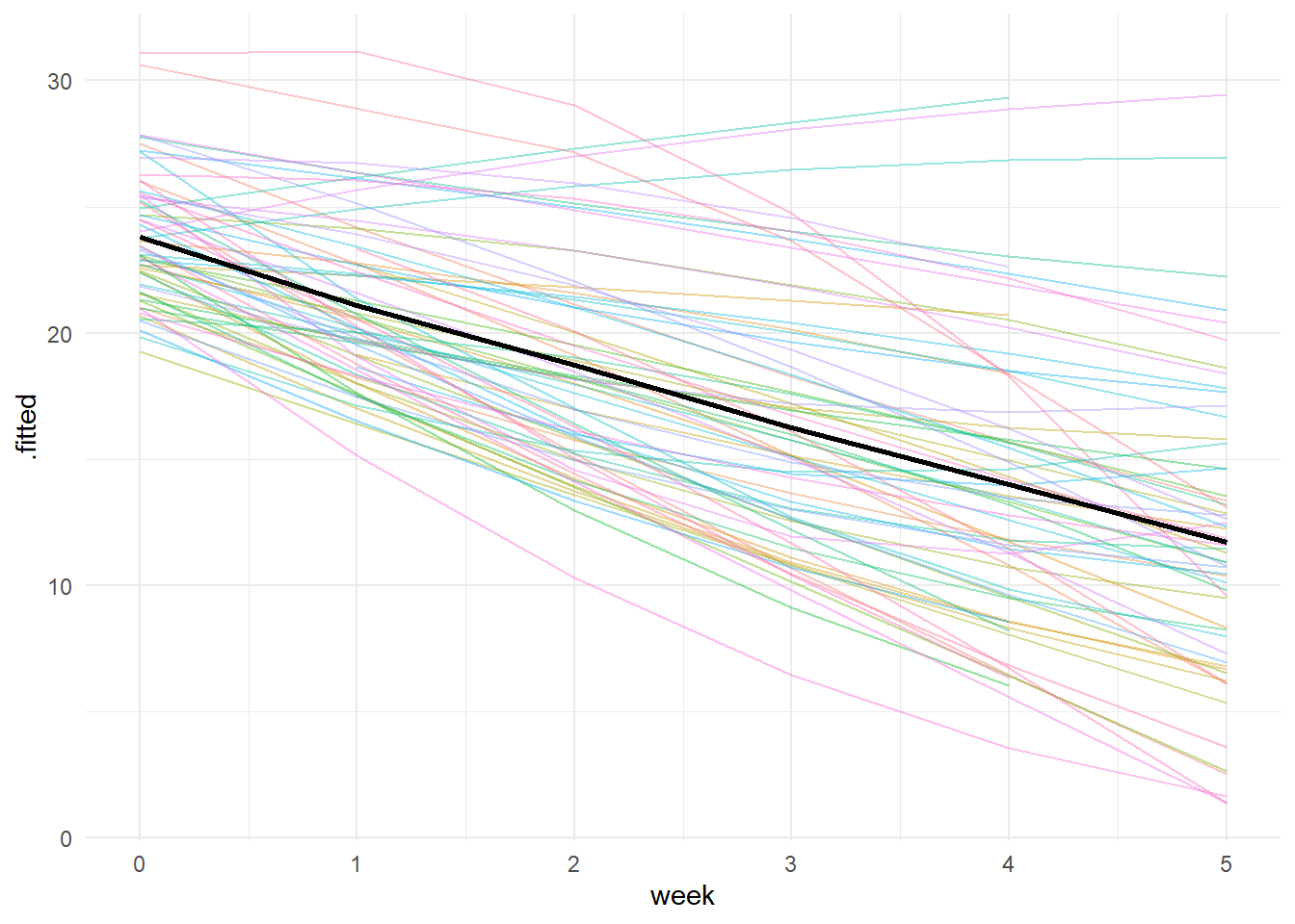
References
Hedeker, Donald; Gibbons, Robert D. (2006). Longitudinal Data Analysis. Wiley.
Maxwell, S. E., Delaney, H. D., & Kelley, K. (2017). Designing experiments and analyzing data: A model comparison perspective. Routledge.
Reisby, N., Gram, L. F., Bech, P., Nagy, A., Petersen, G. O., Ortmann, J., Ibsen, I., Dencker, S. J., Jacobsen, O., Krautwald, O., Søndergaard, I., & Christiansen, J. (1977). Imipramine: Clinical effects and pharmacokinetic variability. Psychopharmacology, 54, 263–272.