One-way ANCOVA

In some situations, a researcher may wish to statistically control for a concomitant variable. A concomitant variable is one that “comes along” with other variables of interest (they are often referred to as covariates). The one-way analysis of covariance (ANCOVA) is one approach that is used to compare means of groups while accounting for a continuous covariate.

The data set

This guide uses data from Chapter 9, Table 7 in the AMCP package. In this hypothetical study, participants are randomly assigned to one of three conditions to examine the effectiveness of a treatment for depression. Participants received a selective serotonin reuptake inhibitor (SSRI) in condition 1, a placebo in condition 2, or were assigned to a wait list control in condition 3. Each participant was also assessed for depression with a pre- and post-treatment inventory. In this type of study, one might want to control for the pre-treatment levels of depression when comparing the three conditions in their post-treatment scores. In this approach, pre-treatment depression scores can serve as covariates to account for baseline levels of depression.

library(tidyverse)
library(AMCP)

# Load data
data(chapter_9_table_7)

# Set the data to a data frame named data instead chapter_9_table_7
# We also set the reference to Condition 3 since it's the wait list control
data <- chapter_9_table_7 %>%
  as_tibble() %>%
  mutate(Condition = factor(Condition))

Generate summary statistics and plots

# Summary statistics
summary_data <- data %>% 
  pivot_longer(cols = Pre:Post, names_to = "Timepoint", values_to = "Score") %>%
  mutate(Timepoint = factor(Timepoint, levels = c("Pre", "Post"))) %>%
  group_by(Condition, Timepoint) %>%
  summarise(
    n = n(),
    min = min(Score),
    max = max(Score),
    median = median(Score),
    mean = mean(Score),
    sd = sd(Score),
    .groups = "drop"
    ) 
    
summary_data %>%
  gt::gt()

Condition	Timepoint	n	min	max	median	mean	sd
1	Pre	10	11	25	16.0	17.0	4.082483
1	Post	10	0	15	9.5	7.3	5.355164
2	Pre	10	11	25	17.0	17.7	5.207900
2	Post	10	3	20	12.5	12.2	5.731007
3	Pre	10	9	29	16.5	17.4	6.310485
3	Post	10	2	25	12.0	14.0	7.571878

Plot Score and Timepoint

data %>% 
  pivot_longer(cols = Pre:Post, names_to = "Timepoint", values_to = "Score") %>%
  mutate(Timepoint = factor(Timepoint, levels = c("Pre", "Post"))) %>%
  ggplot(aes(x = Timepoint, y = Score, color = Condition, fill = Condition)) +
  geom_boxplot(alpha = 0.3) + 
  scale_color_manual(values = c("#440154FF","#1565c0", "#FF9993")) +
  scale_fill_manual(values = c("#440154FF","#1565c0", "#FF9993")) +
  theme_minimal()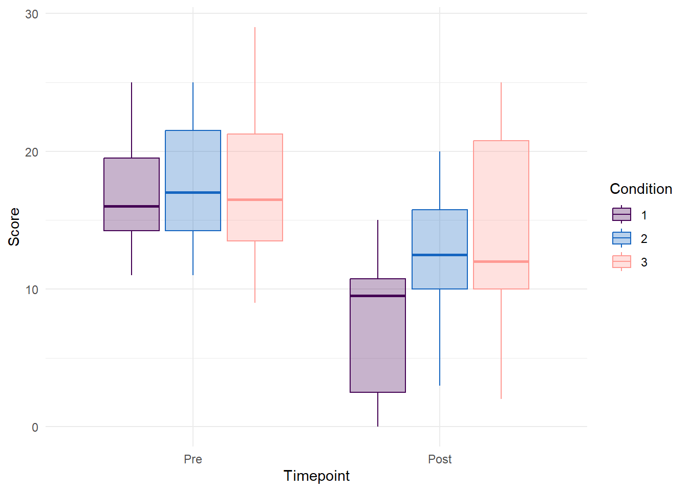

Perform the one-way ANCOVA

The following code chunk represents a way to fit an ANCOVA model using the base R lm() function. The default behavior for R is to set the reference to Condition 1, because it is the first level. However, it may be better to set the reference to Condition 3, the wait list control. This will also mimic the default behavior in SAS. The lm() function can be read as Post test scores predicted by the Pre test scores and Condition.

When we fit the model, we can use the tbl_regression() function from the gtsummary package to display the coefficients. The intercept is interpreted as the predicted value of the outcome when the pre test score = 0 in the reference group (Condition 3). The coefficient for Condition1 is the predicted change from the intercept that can be expected when the pre test score = 0 for those in Condition 1 (2.8 - 6.4 = -3.6). The coefficient for Condition 2 is the predicted change from the intercept that can be expected when the pre test score = 0 for those in Condition 2 (2.8 - 2.0 = -.8).

data <- data %>%
  mutate(Condition = fct_relevel(Condition, "3"))

model <- lm(Post ~ Pre + Condition, data = data)

gtsummary::tbl_regression(model, intercept = TRUE)

Characteristic	Beta	95% CI	p-value
(Intercept)	2.8	-5.1, 11	0.5
Pre	0.65	0.24, 1.0	0.003
Condition
3	—	—
1	-6.4	-11, -1.5	0.013
2	-2.0	-7.0, 3.0	0.4
Abbreviation: CI = Confidence Interval

Lastly, we can retrieve the Type 3 sums of squares table using the Anova() function from the car package to get the results of the F tests. In this context, we focus on the main effects of Pre and Condition. The main effect of Pre can be interpreted as follows: after adjusting for condition Pre score significantly predict Post scores. The main effect of Condition is similarly interpreted as follows: after adjusting for Pre scores, there is a significant difference in Post scores across the 3 conditions. This is analagous to a one-way ANOVA on adjusted means.

aov_tab <- car::Anova(model, type = "III")

# Print out the ANOVA table
aov_tab %>% 
  as.data.frame() %>%
  rownames_to_column(var = "Source") %>%
  gt::gt() %>%
  gt::fmt_number(
    columns = "F value",
    decimals = 2  # Use `decimals` for fixed decimal places
  ) %>%
  gt::fmt(
    columns = c("Pr(>F)"),
    fns = function(x) {
      ifelse(x < 0.001, "< 0.001", formatC(x, format = "f", digits = 3))
    }
  )

Source	Sum Sq	Df	F value	Pr(>F)
(Intercept)	15.29099	1	0.53	0.475
Pre	313.36526	1	10.77	0.003
Condition	217.14948	2	3.73	0.038
Residuals	756.33474	26	NA	NA

Effect sizes for the main effects

We can also display the effect sizes for the main effects of Pre and Condition.

eta_squared <- effectsize::eta_squared(car::Anova(model, type = 3), partial = TRUE)  %>%
  gt::gt() %>%
  gt::fmt_number(
    columns = c("Eta2_partial", "CI_low"),
    decimals = 3  # Use `decimals` for fixed decimal places
  )

eta_squared

Parameter	Eta2_partial	CI	CI_low	CI_high
Pre	0.293	0.95	0.075	1
Condition	0.223	0.95	0.008	1

ANCOVA Plot

An ANCOVA plot can be created by taking advantage of the predict() function to use the regression model to form predictions of the outcome (Post test scores) with the existing pre test and condition values. These predicted values are then added to a column in the primary data frame. Next we relevel the Condition factor to display the Condition legend in numerical order as was displayed in the previous plots. Then pipe the data to a ggplot() call displaying points colored by condition and add an additional layer using the predicted post scores to create a set of lines laid over the raw data points.

data %>%
  mutate(Predicted = predict(model)) %>%
  mutate(Condition = fct_relevel(Condition, c("1", "2", "3"))) %>%
  ggplot(aes(x = Pre, y = Post, color = Condition)) +
  geom_point() +
  geom_line(aes(y = Predicted)) +
  scale_color_manual(values = c("#440154FF","#1565c0", "#FF9993")) +
  theme_minimal()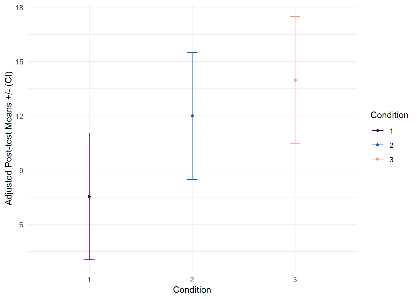

Post hoc tests

For the post hoc tests, we can display the adjusted means for each group. That is, when pre = 0, we can expect the outcome to be 13.98 for condition 3, 7.54 for condition 1, and 11.98 for condition 2. These adjusted means demonstrate higher depression scores in the placebo group, slightly reduced scores in condition 2, and the lowest scores in condition 1 (treated with SSRI). We can then compare these adjusted means in a pairwise fashion to test if Condition 3 is significantly different than Condition 1, Condition 3 is different than Condition 2, and if Condition 2 is different than Condition 1.

# Print estimated marginal means
emms <- emmeans::emmeans(model, ~ Condition) %>%
  as_tibble()

emms %>%
  gt::gt() %>%
  gt::fmt_number(
    columns = c("emmean", "SE", "lower.CL", "upper.CL"),
    decimals = 2  # Use `decimals` for fixed decimal places
  )

Condition	emmean	SE	df	lower.CL	upper.CL
3	13.98	1.71	26	10.47	17.48
1	7.54	1.71	26	4.03	11.05
2	11.98	1.71	26	8.48	15.49

# Plot the adjusted means
emms %>%
  mutate(Condition = fct_relevel(Condition, c("1", "2", "3"))) %>%
  ggplot(aes(y = emmean, x = Condition, color = Condition)) +
  geom_point() +
  geom_errorbar(
    aes(ymin = lower.CL, ymax = upper.CL),
    width = 0.1) +
  scale_color_manual(values = c("#440154FF","#1565c0", "#FF9993")) +
  labs(y = "Adjusted Post-test Means +/- (CI)") +
  theme_minimal()

pwc <- emmeans::emmeans(model, ~ Condition) %>% 
  pairs(adjust = "tukey", infer = c(TRUE, TRUE)) %>%
  as_tibble()
  
# Format the pwc table for display
pwc %>%
  gt::gt() %>%
  gt::fmt_number(
    columns = c("estimate", "SE", "lower.CL", "upper.CL", "t.ratio"),
    decimals = 2  # Use `decimals` for fixed decimal places
  ) %>%
  gt::fmt(
    columns = c("p.value"),
    fns = function(x) {
      ifelse(x < 0.001, "< 0.001", formatC(x, format = "f", digits = 3))
    }
  )

contrast	estimate	SE	df	lower.CL	upper.CL	t.ratio	p.value
Condition3 - Condition1	6.44	2.41	26	0.45	12.44	2.67	0.033
Condition3 - Condition2	1.99	2.41	26	−4.00	7.99	0.83	0.690
Condition1 - Condition2	−4.45	2.42	26	−10.45	1.56	−1.84	0.176

Interpretation

Results from the analysis of covariance revealed a significant relationship between Pre-test and Post-test scores, B = 0.65, SE = 0.2, t(26) = 3.28, p = 0.003 indicating that higher pre-test scores are associated with higher post-test scores after controlling for Condition.

In addition, the analysis revealed a significant main effect for Condition after controlling for Pre-test scores F(2, 26) = 3.73, p = .038, partial η² = .22.

Tukey adjusted post-hoc pairwise comparisons indicate that Post-test depression scores were 6.44 units higher in Condition 3 when compared to Condition 1, t = 2.67, p = 0.033, CI[0.45, 12.44]. No statistically significant differences were observed between Condition 1 and Condition 2 or between Condition 2 and Condition 3.

These results suggest that depression scores are significantly lower in Condition 1 (SSRI) compared to Condition 3 (wait list control), but not significantly lower when compared to Condition 2 (placebo).

References

Maxwell, Scott, Harold Delaney, and Ken Kelley. 2020. AMCP: A Model Comparison Perspective. https://CRAN.R-project.org/package=AMCP.

Maxwell, Scott E, Harold D Delaney, and Ken Kelley. 2017. Designing Experiments and Analyzing Data: A Model Comparison Perspective. Routledge.

Wickham, Hadley. 2019. Tidyverse: Easily Install and Load the ’Tidyverse’. https://CRAN.R-project.org/package=tidyverse.