Two-way Repeated Measures ANOVA

In this guide, I cover how to conduct a repeated measures ANOVA with two within-subjects factors using a univariate approach. The univariate approach can sometimes be referred to as the mixed model approach, but it’s not to be confused with a linear mixed effects model, although linear mixed effects model can and are frequently used to analyze data from research designs with repeated measures.

library(tidyverse)
library(AMCP)

Dataset description

For this guide, we will use the data from Chapter 12 Table 1 in the AMCP package. In this hypothetical study, 10 subjects are participating in an experiment that tests how visual information can interfere with recognizing letters. Each subject performs a letter recognition task in two conditions, noise absent or present. Noise refers to visual information that is presented along with either a letter T or I that the subject needs to identify. Within each condition, visual information was either presented at 0° (directly in front of the participant), at 4° (slightly offset to one side), or at 8° (even more offset to the side). Thus, noise and angle represent our within subjects factors. Finally, the dependent variable in this study is the latency in milliseconds needed to identify the letter.

# Load the data
data(chapter_12_table_1)

# Set to objected named data
data <- chapter_12_table_1

# Display as gt table
data %>%
  format_gt_tbl()

Absent0	Absent4	Absent8	Present0	Present4	Present8
420	420	480	480	600	780
420	480	480	360	480	600
480	480	540	660	780	780
420	540	540	480	780	900
540	660	540	480	660	720
360	420	360	360	480	540
480	480	600	540	720	840
480	600	660	540	720	900
540	600	540	480	720	780
480	420	540	540	660	780

Prepare the data (wide to long)

The data set from the package is in a wide format. Re-arranging the data set so that it is in long format will facilitate model fitting, summarizing data, and generating figures.

rm_data <- data %>%
  mutate(id = as.character(seq(1:dim(data)[1]))) %>%
  group_by(id) %>%
  pivot_longer(cols = -id, values_to = "latency",  names_to  = "condition.angle") %>%
  ungroup() %>%
  separate(col = condition.angle,
           into = c("condition", "angle"),
           sep = -1) %>%
  mutate(across(condition:angle, ~ factor(.x)))

Here’s a view of the first several rows of the long format data. In this format, each subject should have 6 rows of data, one for each combination of condition and angle.

id	condition	angle	latency
1	Absent	0	420
1	Absent	4	420
1	Absent	8	480
1	Present	0	480
1	Present	4	600
1	Present	8	780

Generate summary statistics

Next we generate summary statistics to inspect the data focusing on marginal (averaged over one factor) and cell means (averaged over combinations of the factors).

Summary for angle

Once the data is in long format, we can group it by angle and summarize it using a custom function I wrote using the dplyr package.

rm_data %>% 
  group_by(angle) %>%
  summarize_column(latency) %>%
  format_gt_tbl()

angle	n	min	max	median	mean	sd	se
0	20	360	660	480	477	74.06	16.56
4	20	420	780	600	585	122.92	27.49
8	20	360	900	600	645	154.36	34.52

Summary for condition

Similarly, we can group the data by the noise condition and calculate the marginal means.

rm_data %>% 
  group_by(condition) %>%
  summarize_column(latency) %>%
  format_gt_tbl()

condition	n	min	max	median	mean	sd	se
Absent	30	360	660	480	500	77.73	14.19
Present	30	360	900	660	638	152.35	27.81

Summary for combinations of condition and angle

Finally, we can group by condition and angle to calculate cell means.

summary_data <- rm_data %>% 
  group_by(condition, angle) %>%
  summarize_column(latency)
    
summary_data %>% 
  format_gt_tbl()

condition	angle	n	min	max	median	mean	sd	se
Absent	0	10	360	540	480	462	56.92	18.00
Absent	4	10	420	660	480	510	86.02	27.20
Absent	8	10	360	660	540	528	78.99	24.98
Present	0	10	360	660	480	492	88.54	28.00
Present	4	10	480	780	690	660	109.54	34.64
Present	8	10	540	900	780	762	116.79	36.93

Plot the data

Next, we can plot the data to reveal any patterns or trends and to visualize the distribution of the dependent variables.

Box plots

One option to visualize the data is through box plots for each angle where each condition is displayed in a separate panel. In this figure, means are indicated by a diamond.

rm_data %>%
ggplot(aes(x = angle, y = latency, color = angle, fill = angle)) +
  geom_boxplot(alpha = 0.1) +
  stat_summary(fun = mean, geom = "point", shape = 5, size = 3, stroke = 1) +
  scale_color_manual(values = c("#440154FF","#1565c0", "#FF9993")) +
  scale_fill_manual(values = c("#440154FF","#1565c0", "#FF9993")) +
  facet_wrap(~ condition) +
  labs(y = "Latency (ms)", x = "Angle") +
  theme_minimal() + 
  theme(legend.position = "none")

Line plots

We could also focus on the cell means and plot them in a line plot.

summary_data %>%
  ggplot(aes(x = angle, y = mean, group = condition, color = condition)) +
  geom_line(alpha = 0.5) +
  geom_point() +
  labs(y = "Latency (ms)", x = "Angle", color = "Condition") +
  theme_minimal()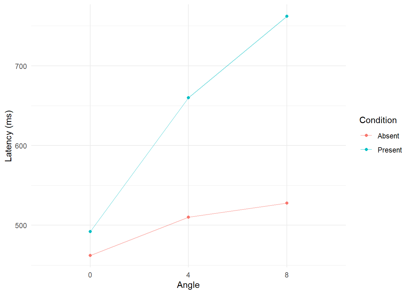

Perform two-way repeated measures ANOVA (univariate approach)

In this approach the model can be fit using the base R aov() function.

model <- aov(latency ~ angle * condition + Error(id/(angle*condition)), data = rm_data)

summary(model)

For this design, the output of summary(model) is a list with 4 elements. The first element contains output for the residuals of the error term for id. Elements 2, 3, and 4 contain output for the main effects for condition, angle, and the interaction between condition and angle respectively. Since elements 2 through 4 contain the main effects, I created a helper function that takes in as input a vector of the elements we want to display.

c(2, 3, 4) %>%
  purrr::map_df(
    ., 
    ~ summary(model)[[.x]][[1]] %>%
        as.data.frame() %>% 
        mutate(Source = rownames(.)) %>%
        select(Source, everything())
  ) %>%
  format_gt_tbl()

Source	Df	Sum Sq	Mean Sq	F value	Pr(>F)
angle	2	289920	144960	40.72	< 0.001
Residuals	18	64080	3560	NA	NA
condition	1	285660	285660	33.77	< 0.001
Residuals	9	76140	8460	NA	NA
angle:condition	2	105120	52560	45.31	< 0.001
Residuals	18	20880	1160	NA	NA

Interpretation of main effects

A two-way repeated measures ANOVA revealed a significant effect of angle F(2, 18) = 40.72, p < 0.001 suggesting that the marginal means of each level of angle are not equal to one another. In addition, the analysis revealed a significant effect of condition F(1, 9) = 33.77, p < 0.001 suggesting that mean latency scores were overall higher in the present condition compared to absent. Finally, a significant angle by condition interaction was observed F(2, 18) = 45.31, p < 0.001 indicating the the effect of condition is not the same at each level of angle. In order to shed light on the interaction simple-effects analyses were conducted.

Effect of angle within each level condition

In the case of angle within each level of condition, we can conduct two separate one-way repeated measures ANOVAs, one for a subset of data from the absent condition and another for a subset of data from the present condition. To control for family wise error rate, a Bonferroni (.05/2, or 0.025) adjustment was implemented. These results reveal a significant simple effect of angle within the absent condition F(2,18) = 5.05, p = 0.018 and angle within the present condition F(2, 18) = 77.02, p < 0.001.

c("Absent", "Present") %>%
  purrr::map_df(
    .,
    ~ summary(aov(latency ~ angle + Error(id/angle),
    data = (rm_data %>% filter(condition == .x))))[[2]][[1]] %>%
    as.data.frame() %>%
    drop_na()    
  ) %>%
  mutate(Source = c("Angle w/in Absent", "Angle w/in Present")) %>%
  select(Source, everything()) %>%
  format_gt_tbl()

Source	Df	Sum Sq	Mean Sq	F value	Pr(>F)
Angle w/in Absent	2	23280	11640	5.05	0.018
Angle w/in Present	2	371760	185880	77.02	< 0.001

Pairwise comparisons

Next, we follow up the significant simple-effects with pairwise comparisons of each level of angle within each condition. To control for the family wise error rate, we use a Bonferroni adjustment where the p-value threshold determined by .025/3 (0.0083).

em <- emmeans::emmeans(model, ~ angle | condition)

Note: re-fitting model with sum-to-zero contrasts

# Since we are performing our on p-value adjustment, set adjust to "none"
# Could also set adjust = "bonferroni" and use alpha = 0.05.
emmeans::contrast(em, method = "pairwise", adjust = "none") %>%
  as.data.frame() %>%
  format_gt_tbl()

contrast	condition	estimate	SE	df	t.ratio	p.value
angle0 - angle4	Absent	-48	21.73	28.60	−2.21	0.035
angle0 - angle8	Absent	-66	21.73	28.60	−3.04	0.005
angle4 - angle8	Absent	-18	21.73	28.60	−0.83	0.414
angle0 - angle4	Present	-168	21.73	28.60	−7.73	< 0.001
angle0 - angle8	Present	-270	21.73	28.60	−12.43	< 0.001
angle4 - angle8	Present	-102	21.73	28.60	−4.69	< 0.001

The results indicate that at the level of condition absent, there is one significant difference after Bonferroni adjustment suggesting that mean latencies are higher at angle 8 compared to angle 0 t(28.6) = 3.04, p = 0.005. At the level of condition present, all pairwise comparisons are significantly different such that angle 0 is 168 units lower than angle 3 t(28.6) = -7.73, p < 0.001, angle 0 is 270 units lower than angle 8 t(28.6) = -12.43, p < 0.001, and angle 4 is 102 units lower than angle 8 t(28.6) = -4.69, p <0.001. Taken together, the results suggest that in the absent condition, angle has a limited and week effect whereas in the present condition, angle has a stronger and more widespread effect.

summary_data %>%
  ggplot(aes(x = condition, y = mean, group = angle, color = angle)) +
  geom_line() +
  geom_point() +
  geom_errorbar(aes(ymin = mean - se, ymax = mean + se, width = 0.1)) +
  scale_color_manual(values = c("#440154FF","#1565c0", "#FF9993")) +
  labs(x = "Condition", y = "Latency (ms)", color = "Angle") +
  theme_minimal()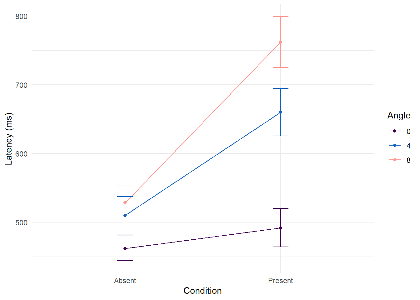

Effect of condition within each level of angle

In the case of condition within each level of angle, we can conduct three separate one-way repeated measures ANOVAs. To control for family wise error rate, a Bonferroni (.05/3, or 0.017) adjustment was implemented. These results reveal significant simple-effects of condition within angle 4 F(1,9) = 19.74, p = 0.002 and condition within angle 8 F(1, 9) = 125.59, p < 0.001. In each of these comparisons mean latencies from the present condition were higher than those in the absent condition. Since condition is only two levels, not further pairwise comparisons are needed.

c("0", "4", "8") %>%
  purrr::map_df(
    .,
    ~ summary(aov(latency ~ condition + Error(id/condition),
    data = (rm_data %>% filter(angle == .x))))[[2]][[1]] %>%
    as.data.frame() %>%
    drop_na()    
  ) %>%
  mutate(Source = c("Condition w/in 0", "Condition w/in 4",  "Condition w/in 8")) %>%
  select(Source, everything()) %>%
  format_gt_tbl()

Source	Df	Sum Sq	Mean Sq	F value	Pr(>F)
Condition w/in 0	1.000	4500	4500	1.55	0.244
Condition w/in 4	1.000	112500	112500	19.74	0.002
Condition w/in 8	1.000	273780	273780	125.59	< 0.001

summary_data %>%
  ggplot(aes(x = angle, y = mean, group = condition, color = condition)) +
  geom_line() +
  geom_point() +
  geom_errorbar(aes(ymin = mean - se, ymax = mean + se, width = 0.1)) +
  labs(y = "Latency (ms)", x = "Angle", color = "Condition") +
  theme_minimal()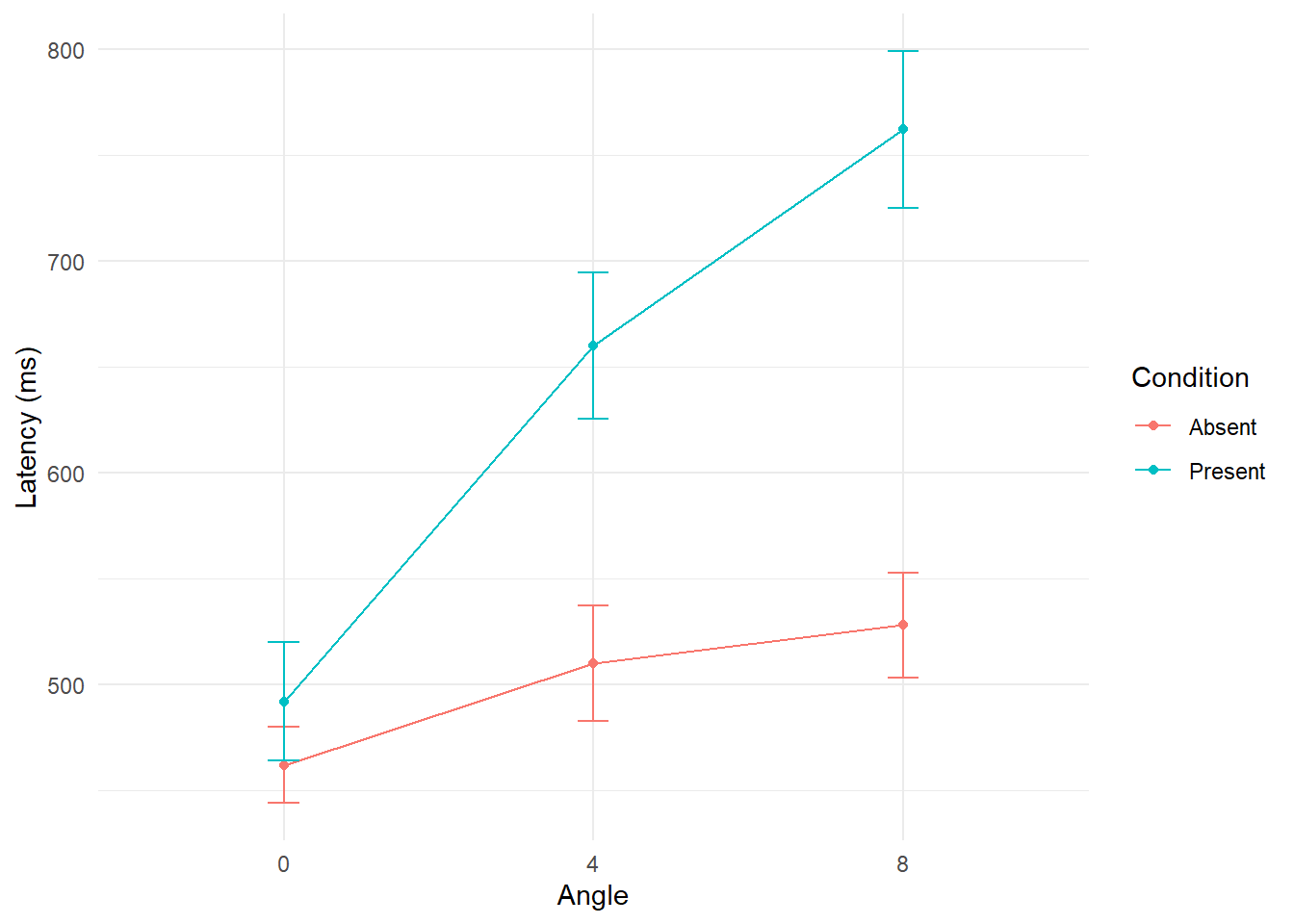

Two-way repeated measures ANOVA in a linear mixed effect regression (lmer) model framework

We use the lmerTest package and the lmer() function to fit a linear mixed-effects model. The lme4 package can also be used to fit the same model, as the syntax is identical. However, lme4 does not provide p-values by default, for principled reasons related to the complexity of estimating degrees of freedom in mixed models.

In this model, we are predicting latency as a function of angle, condition, and their interaction. These are treated as fixed effects. The term (1 | id) specifies a random intercept for each subject, allowing each participant to have their own baseline latency. The terms (1 | condition:id) and (1 | angle:id) allow for random variation in how each subject responds to each condition and each angle, respectively. These account for subject-specific deviations from the average effects of condition and angle.

A term like (1 | id:angle:condition) is not included because the variability it would capture is already modeled through the combination of the existing random effects. Including it would be redundant and potentially overfit the model, especially with a modest sample size.

lmer_model <- lmerTest::lmer(
  latency ~ angle + condition + angle:condition + (1|id) + (1|condition:id) + (1|angle:id), 
  data = rm_data)

Display the type 3 tests of fixed effects table

anova(lmer_model)

Effect	Sum Sq	Mean Sq	NumDF	DenDF	F value	Pr(>F)
angle	94,468.26	47,234.13	2	18.00	40.72	< 0.001
condition	39,168.58	39,168.58	1	9.00	33.77	< 0.001
angle:condition	105,120.00	52,560.00	2	18.00	45.31	< 0.001

Display solution for fixed effects

As in the approach for the one-way ANOVA, we can use the broom.mixed package to display the model output for the main effects. In the model specification with two categorical factors, condition absent angle 0 is the reference group. All other estimates are interpreted in relation to the reference group.

broom.mixed::tidy(mer_model)

term	estimate	std.error	statistic	df	p.value
(Intercept)	462	28.97	15.95	19.79	< 0.001
angle4	48	21.73	2.21	28.60	0.035
angle8	66	21.73	3.04	28.60	0.005
conditionPresent	30	26.81	1.12	14.08	0.282
angle4:conditionPresent	120	21.54	5.57	18.00	< 0.001
angle8:conditionPresent	204	21.54	9.47	18.00	< 0.001

The estimate for the intercept represents the mean latency for the absent condition at angle 0. The estimate for angle4 (48) represents the difference between the mean of absent angle 0 and absent angle 4. We can calculated the mean latency for the absent condition at angle 4 by summing 462 and 48 which yields 510 and is the group mean displayed in the summary statistics table above. The p-value for angle 4 corresponds to a test of the difference between absent angle 4 and the reference absent angle 0.

The estimate for angle8 (66) represents the difference between the mean of absent angle 0 and absent angle 8. We can obtain the mean of absent angle 8 by summing 462 (intercept) and 66 which yields 528 (also in the summary statistics table above). As in the previous estimate, the p-value corresponds to a test of of the difference between absent angle 0 and absent angle 8.

The estimate for the conditionPresent term represents the average difference between absent angle 0 and present angle 0. In other words, it is the effect of condition at angle 0. This estimate is not significant p = 0.282 suggesting that there is no difference between the two conditions at angle 0.

We’ve established that the effect of condition at angle 0 (the reference) is an increase of 30 ms. The estimate for conditionPresent:angle4 (120) represents how much larger the effect of condition is at angle 4 compared to angle 0. The mean latency for angle 4 when condition is absent is given by summing 462 (intercept) and 48 (angle4) which equals 510. The mean latency for angle 4 when condition is present is given by summing 462 (intercept), 48 (angle4), 30 (conditionPresent), and 120 (angle4:conditionPresent) which equals 660. The effect of condition at angle 4 is 660 − 510 = 150. Now we compare the effect of condition at angle 0 and the effect of condition at angle 4. The effect of condition is 150 at angle 4 versus 30 at angle 0, a difference of 120. This corresponds to the interaction term. In other words, the coefficient can be interpreted as a difference in differences, showing that the effect of condition is significantly greater at angle 4 than at angle 0.

The estimate for the conditionPresent:angle8 term (204) represents the additional latency in present angle 8 compared to absent angle 8. The effect for condition present is 30 and the effect of conditionPresent:angle8 is 204. This sums to 234 which represents the difference between the mean latency of absent angle 8 (528) and present angle 8 (762). Again this estimate tests for the additional increase in latency when both condition is present and angle is 8.

Simple effects

Effect of angle within each level of condition

c("Absent", "Present") %>%
  purrr::map_df(
    .,
    ~ anova(lmerTest::lmer(
        latency ~ angle + (1|id), 
        data = (rm_data %>% filter(condition == .x)))) %>%
        as.data.frame() %>%
        mutate(Effect = rownames(.)) %>%
        select(Effect, everything())
  ) %>%
  mutate(Effect = c("Angle w/in Absent", "Angle w/in Present")) %>%
  select(Effect, everything()) %>%
  format_gt_tbl()

Effect	Sum Sq	Mean Sq	NumDF	DenDF	F value	Pr(>F)
Angle w/in Absent	23280	11640	2	18.00	5.05	0.018
Angle w/in Present	371760	185880	2	18.00	77.02	< 0.001

To obtain the pairwise differences between each level of angle within each level of condition we simply switch the order of the main effects in the emmeans() function. If we use the adjust = “none” option, the t.ratio and p.value from the contrast angle0 - angle4 and angle - angle8 contrats will match the model output for the angle4 and angle8 terms. If the adjust = “none” option is omitted, then the resulting p.values will change but the t.ratio will not.

em <- emmeans::emmeans(lmer_model, ~ angle | condition)

emmeans::contrast(em, method = "pairwise", adjust = "none") %>%
  as.data.frame() %>%
  format_gt_tbl()

contrast	condition	estimate	SE	df	t.ratio	p.value
angle0 - angle4	Absent	-48	21.73	28.60	−2.21	0.035
angle0 - angle8	Absent	-66	21.73	28.60	−3.04	0.005
angle4 - angle8	Absent	-18	21.73	28.60	−0.83	0.414
angle0 - angle4	Present	-168	21.73	28.60	−7.73	< 0.001
angle0 - angle8	Present	-270	21.73	28.60	−12.43	< 0.001
angle4 - angle8	Present	-102	21.73	28.60	−4.69	< 0.001

Effect of condition within each level of angle

c("0", "4", "8") %>%
  purrr::map_df(
    .,
    ~ anova(lmerTest::lmer(
        latency ~ condition + (1|id), 
        data = (rm_data %>% filter(angle == .x)))) %>%
        as.data.frame() %>%
        mutate(Effect = rownames(.)) %>%
        select(Effect, everything())
  ) %>%
  mutate(Effect = c("Condition w/in 0", "Condition w/in 4",  "Condition w/in 8")) %>%
  select(Effect, everything()) %>%
  format_gt_tbl()

Effect	Sum Sq	Mean Sq	NumDF	DenDF	F value	Pr(>F)
Condition w/in 0	4500	4500	1.000	9.00	1.55	0.244
Condition w/in 4	112500	112500	1.000	9.00	19.74	0.002
Condition w/in 8	273780	273780	1.000	9.00	125.59	< 0.001

# em <- emmeans::emmeans(mer_model, ~ condition | angle)

# emmeans::contrast(em, method = "pairwise") %>%
#   as.data.frame() %>%
#   format_gt_tbl()

References

Maxwell, Scott, Harold Delaney, and Ken Kelley. 2020. AMCP: A Model Comparison Perspective. https://CRAN.R-project.org/package=AMCP.

Maxwell, Scott E, Harold D Delaney, and Ken Kelley. 2017. Designing Experiments and Analyzing Data: A Model Comparison Perspective. Routledge.

Wickham, Hadley. 2019. Tidyverse: Easily Install and Load the ’Tidyverse’. https://CRAN.R-project.org/package=tidyverse.