One-way ANOVA

Data set description

This guide relies on a data set from Exercise 9 in Chapter 3 of the AMCP package. AMCP is the accompanying package for Maxwell, Delaney, & Kelley’s “Designing Experiments and Analyzing Data: A Model Comparison Perspective.”

In this exercise, a psychologist randomly assigned 12 subjects to one of 4 different therapy treatments. These treatments consisted of rational-emotive, psychoanalytic, client-centered, and behavioral therapies coded as 1 through 4 respectively. The 4 different treatments were used to investigate which therapy is more effective at reducing phobia scores.

For these data, Group represents the type of therapy the participant was assigned to. Scores represent the outcome variable from a post-therapy fear scale where higher numbers indicate higher levels of phobia. Finally, the data are arranged in a manner so that each row represents the group and scores for one subject.

Code for one-way ANOVA

Load Packages

library(tidyverse)
library(AMCP)
library(multcomp)

Approach

There are several ways to conduct a one-way ANOVA in R each with it’s own advantages and disadvantages. There are some very nice covenience functions available in packages such as rstatix, ezANOVA, and jmv that can simplify running one-way ANOVAs. However, they may not always be as flexible as desired when working with real world data. In addition, the output from these packages is not always well suited for display in quarto documents. For these reasons, I’ve chosen to stick to base R functions as much as possible and modifying the output for display in Quarto documents.

Prepare the data

For this approach we will want to convert the Group variable into a factor (categorical variable) to prevent R from treating it as a numerical variable. We will also assume that the assumptions of independence, equality of variance, and normality are met for the sample data set.

# Load the data
data(C3E9)

data <- C3E9

# Convert Group to factor
data <- 
  data %>% 
  mutate(Group = factor(case_match(Group,
    1 ~ "RE",
    2 ~ "PA",
    3 ~ "CC", 
    4 ~ "BT")))
  # Group = factor(Group, levels = c(1, 2, 3, 4)))

# Display the data
data %>%
  gt::gt()

Group	Scores
RE	2
RE	4
RE	6
PA	10
PA	12
PA	14
CC	4
CC	6
CC	8
BT	8
BT	10
BT	12

Generate summary statistics

It’s always a good idea to generate summary statistics to get an overall picture of the data and identify potential issues such as outliers, missing values, and other abnormalities.

# Summary statistics
data %>% 
  group_by(Group) %>%
  summarise(
    n = n(),
    min = min(Scores),
    max = max(Scores),
    median = median(Scores),
    mean = mean(Scores),
    sd = sd(Scores)   
    ) %>%
  gt::gt()

Group	n	min	max	median	mean	sd
BT	3	8	12	10	10	2
CC	3	4	8	6	6	2
PA	3	10	14	12	12	2
RE	3	2	6	4	4	2

Plot the data

Next, we may want to plot the data to get a visual sense of any patterns.

data %>%
  ggplot(aes(x = Group, y = Scores)) +
  geom_boxplot() +
  theme_minimal()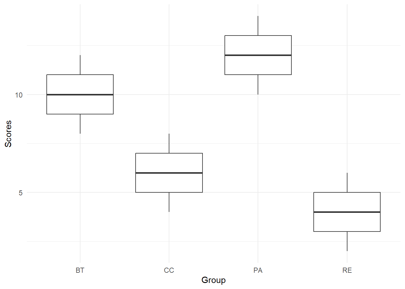

Perform the one-way ANOVA

To perform the one-way ANOVA, I will first fit a linear model. We then use the car (companion to applied regression) package to display the results and to specify the use of Type 3 sums of squares.

# Specify an lm() model
model <-  lm(Scores ~ Group, data = data)

aov_tab <- car::Anova(model, type = "III")

# Print out the ANOVA table
aov_tab %>% 
  as.data.frame() %>%
  rownames_to_column(var = "Source") %>%
  gt::gt() %>%
  gt::fmt_number(
    columns = "Pr(>F)",
    decimals = 4  # Use `decimals` for fixed decimal places
  ) %>%
  gt::fmt(
    columns = c("Pr(>F)"),
    fns = function(x) {
      ifelse(x < 0.001, "< 0.001", formatC(x, format = "f", digits = 3))
    }
  )

Source	Sum Sq	Df	F value	Pr(>F)
(Intercept)	300	1	75	< 0.001
Group	120	3	10	0.004
Residuals	32	8	NA	NA

Post hoc tests

To get the output for the post hoc tests, we will run the glht() function on the model object and specifying linfct as Group = “Tukey”. From there summary(tukey_glht) will display the results in the console. To get a table to display in a report, additional coding is needed to transform the glht() object to a data frame. From there the row names need to be manipulated and the columns re-ordered. Next the column names are cleaned up before passing the data frame to gt() where the digits can be formatted.

Tukey’s Honest Significant Difference (HSD)

tukey_glht <- glht(model, linfct = mcp(Group = "Tukey"))

# Extract the values of interest and convert to data frame
tukey_df <- as.data.frame(
  summary(tukey_glht)$test[c("coefficients", "sigma", "tstat", "pvalues")]
  )

# Display table
tukey_df %>%
  rownames_to_column(var = "Comparison") %>%
  rename(
    "Estimate" = "coefficients",
    "SE" = "sigma") %>%
  gt::gt() %>%
  gt::fmt_number(
    columns = c(SE, tstat, pvalues),
    decimals = 2  # Use `decimals` for fixed decimal places
  ) %>%
  gt::fmt(
    columns = c(pvalues),
    fns = function(x) {
      ifelse(x < 0.001, "< 0.001", formatC(x, format = "f", digits = 3))
    }
  )

Comparison	Estimate	SE	tstat	pvalues
CC - BT	-4	1.63	−2.45	0.144
PA - BT	2	1.63	1.22	0.630
RE - BT	-6	1.63	−3.67	0.026
PA - CC	6	1.63	3.67	0.026
RE - CC	-2	1.63	−1.22	0.630
RE - PA	-8	1.63	−4.90	0.005

Interpret the output

A one-way analysis of variance (ANOVA) revealed a significant effect of Group on phobia scores, F(3, 8) = 10.00, p < 0.05, indicating that mean scores differed across the four treatment conditions. Post hoc pairwise comparisons using the Tukey’s HSD demonstrated that phobia scores were significantly lower following rational-emotive therapy (Group 1) compared to both psychoanalytic therapy (Group 2) and behavioral therapy (Group 4). Additionally, phobia scores following client-centered therapy (Group 3) were significantly lower than those following psychoanalytic therapy (Group 2). These findings suggest that rational-emotive and client-centered therapies were associated with greater reductions in phobia scores relative to psychoanalytic therapy.

References

Maxwell, Scott, Harold Delaney, and Ken Kelley. 2020. AMCP: A Model Comparison Perspective. https://CRAN.R-project.org/package=AMCP.

Maxwell, Scott E, Harold D Delaney, and Ken Kelley. 2017. Designing Experiments and Analyzing Data: A Model Comparison Perspective. Routledge.

Wickham, Hadley. 2019. Tidyverse: Easily Install and Load the ’Tidyverse’. https://CRAN.R-project.org/package=tidyverse.