library(tidyverse)
library(AMCP)
library(multcomp)
library(dfmtbx)Welch’s ANOVA
When the homogeneity of variance assumption is violated in a one-way ANOVA, a Welch’s ANOVA can be conducted in place. However, one limitation for the Welch’s ANOVA is that it is restricted to data with only one independent variable or factor (i.e. one-way between-subjects designs). The following covers how to test for normality, homogeneity of variance and how to conduct a Welch’s ANOVA. The same example data from the one-way ANOVA are used here.
Prepare the data
# Load the data
data(C3E9)

data <- C3E9

# Convert Group to factor
data <-
  data %>%
  mutate(Group = factor(case_match(Group,
    1 ~ "RE",
    2 ~ "PA",
    3 ~ "CC",
    4 ~ "BT")))
  # Group = factor(Group, levels = c(1, 2, 3, 4)))

# Display the data
data %>%
format_gt_tbl()| Group | Scores |
|---|---|
| RE | 2 |
| RE | 4 |
| RE | 6 |
| PA | 10 |
| PA | 12 |
| PA | 14 |
| CC | 4 |
| CC | 6 |
| CC | 8 |
| BT | 8 |
| BT | 10 |
| BT | 12 |
Check normality
To produce the Shapiro-Wilk’s test of normality, we will need to create an analysis of variance (aov) object with the base R aov() function. In the code chunk below, the aov object is piped to the residuals() function, which is then piped to the shapiro.test() function. This will conduct Shapiro-Wilk’s test on the residuals of the aov object and not the observed values of the dependent variable. Our Shaprio-Wilk’s test result, W = 0.81 is significant with a p-values less than 0.05 which is taken as evidence that our data violate the assumption of normality.
In addition to the Shapiro-Wilk test, we can visualize the residuals of our data and plot them against the expected residuals of a normal distribution. If our data are normally distributed, we would expect the individual data points to hover near the diagonal line. As we can see in the plot, we have quite a few data points fall far away from the line which is additional evidence that our data are not normally distributed. When the assumption of normality is violated one can explore the use of a robust ANOVA.
# Base R Shapiro-Wilk test on residuals of the aov object
aov(Scores ~ Group, data = data) %>%
  residuals() %>%
  shapiro.test()
    Shapiro-Wilk normality test

data:  .
W = 0.81079, p-value = 0.01246
# Create a plot of standardised residuals, indexed at position 2 of plot(aov(x))
plot(aov(formula = Scores ~ Group, data = data), 2)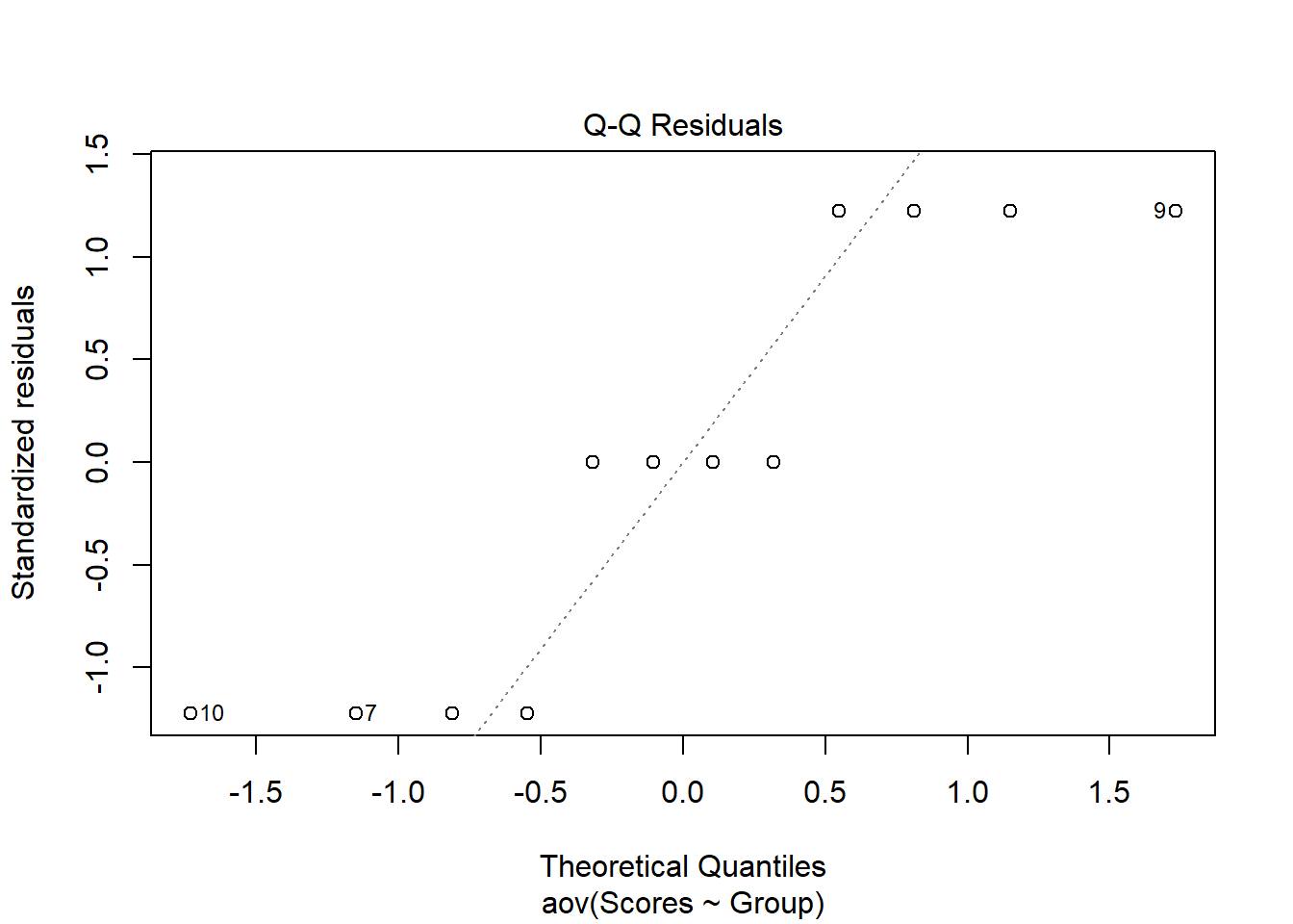
Check homogeneity of variance
Finally, for the homogeneity of variance test, the leveneTest() function from the car package can accomplish this task. The result is not-significant which indicates that the data meet the assumption of homogeneity of variance.
As in the examination of normality above, base R also can also plot the Residuals vs Fitted values to examine homogeneity of variance. The plot maintains a straight red line which is what would be expected for data that meet the homogeneity of variance assumption.
results <- car::leveneTest(Scores ~ Group, data = data)| Df | F value | Pr(>F) |
|---|---|---|
| 3 | 0.0000 | 1.000 |
# Residuals vs Fitted values plot
plot(aov(formula = Scores ~ Group, data = data), 1)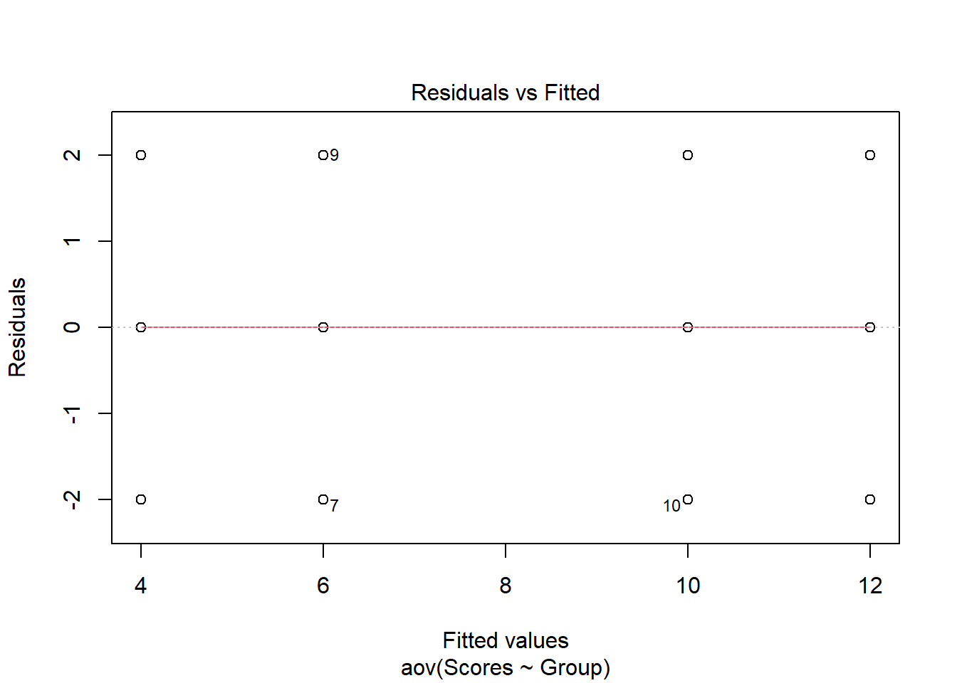
Perform the Welch’s one-way ANOVA
To perform the Welch’s one-way ANOVA, we use the oneway.test() function from base R. We’ll save the results to an oject that we can use to create and then format a table for display.
results <- oneway.test(Scores ~ Group, data = data, var.equal = FALSE)| Source | F value | Pr(>F) |
|---|---|---|
| Group | 7.69 | 0.032 |