One-way repeated measures ANOVA

library(tidyverse)
library(AMCP)

Data set description

Repeated measures ANOVAs are used in cases where observations from the same unit(participant, animal subject) are captured multiple times. An example of this type of experimental design comes from the Table 5 of Chapter 11 from the AMCP package. The data represent are from a hypothetical study that tracked the age-normed general cognitive scores from the McCarthy Scales of Children’s Abilities (MSCA) of 12 children at 4 different time points (age at 30, 36, 42, and 48 months). As displayed below, these data are well behaved in the sense that there are no missing values, each subject has the same number of data points, and the time intervals between measurements are equally spaced. A repeated measures ANOVA is one option to analyze these data.

# Load the data
data("chapter_11_table_5")

# Set to objected named data
data <- chapter_11_table_5

# Display as table
data %>%
  format_gt_tbl()

Months30	Months36	Months42	Months48
108	96	110	122
103	117	127	133
96	107	106	107
84	85	92	99
118	125	125	116
110	107	96	91
129	128	123	128
90	84	101	113
84	104	100	88
96	100	103	105
105	114	105	112
113	117	132	130

Prepare the data (wide to long)

Before proceeding, we will create a column with values that represent the subject id number. Since this is an indentification number and doesn’t represent a quantity, we will also want to convert the id column to factor or character format. Lastly, we then convert the data set to long format using the pivot_longer() function. Pivoting the data to long format will facilitate analyses, plotting, and summarizing values.

rm_data <- data %>%
  mutate(id = as.character(seq(1:dim(data)[1]))) %>%
  group_by(id) %>%
  pivot_longer(cols = Months30:Months48, values_to = "score",  names_to  = "age") %>%
  ungroup()

Here’s a view of the first several rows of the long format data. In this format, each subject should have 4 rows of data, one for each timepoint.

rm_data %>%
  head() %>%
  format_gt_tbl()

id	age	score
1	Months30	108
1	Months36	96
1	Months42	110
1	Months48	122
2	Months30	103
2	Months36	117

Generate summary statistics

Next we will generate some summary statistics to inspect the data.

rm_data %>% 
  group_by(age) %>%
  summarise(
    n = n(),
    min = min(score),
    max = max(score),
    median = median(score),
    mean = mean(score),
    sd = sd(score)   
    ) %>%
  format_gt_tbl()

age	n	min	max	median	mean	sd
Months30	12	84	129	104.00	103	13.71
Months36	12	84	128	107.00	107	14.16
Months42	12	92	132	105.50	110	13.34
Months48	12	88	133	112.50	112	14.76

Plot the data

We can also plot the data using the id as a grouping variable so that each line represents an individual subject.

rm_data %>%
  ggplot(aes(x = age, y = score, group = id, color = id)) +
  geom_line(alpha = 0.5) +
  theme_minimal() + 
  theme(legend.position = "none")

Another option is to plot the quartiles with boxplots to gain a visual sense of the distribution. In the following code chunk, I also added a stat_summary() call to plot the means of each time point.

rm_data %>%
  ggplot(aes(x = age, y = score, color = age, fill = age)) +
  geom_boxplot(alpha = 0.5) +
  stat_summary(fun = mean, geom = "point", shape = 5, size = 3, stroke = 1) +
  theme_minimal() + 
  theme(legend.position = "none")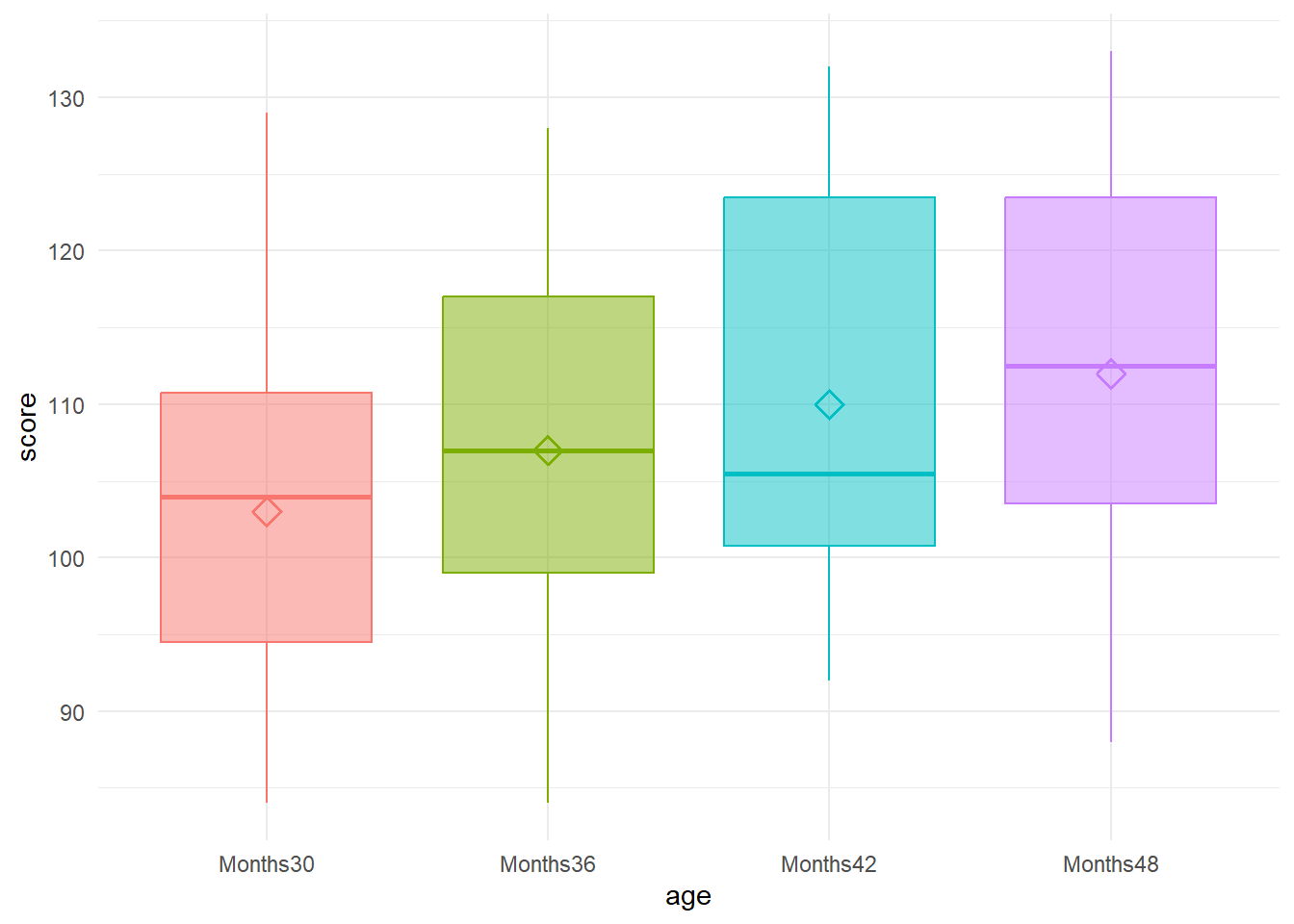

Perform the one-way repeated measures ANOVA

To perform the one-way repeated measures ANOVA, we will rely on the aov() function and specify a model where score is predicted by age and an error term. The error term (Error(id/age)) indicates that age is a repeated measure within each subject id. After fitting the model, summary(model) can be used to display the model output. With some targeted indexing of the model output (summary(model)[[2]][[1]]), a table of the univariate tests of within subjects effects can be displayed in a .qmd document.

# This will match SAS proc glm with wide data structure
model <- aov(score ~ age + Error(id/age), data = rm_data)

summary(model)

Source	Df	Sum Sq	Mean Sq	F value	Pr(>F)
age	3	552	184.00	3.03	0.043
Residuals	33	2006	60.79	NA	NA

In this case, the interpretation of the RM-ANOVA results is analogous to the interpretation of omnibust test of the one-way between subjects ANOVA. There is a significant main effect which indicates that there is at least one significant difference between any two time points of age. To determine, where this difference lies, we can conduct post-hoc tests.

Post-hoc tests

Here, we test every pairwise combination of time points and display the Tukey adjusted p values. The only significant difference between timepoints is between 30 and 48 months.

# Get estimated marginal means
em <- emmeans::emmeans(model, ~ age)

# Tukey adjusted pairwise comparisons
pairs(em) %>%
  as.data.frame() %>%
  format_gt_tbl()

contrast	estimate	SE	df	t.ratio	p.value
Months30 - Months36	-4	3.18	33	−1.26	0.596
Months30 - Months42	-7	3.18	33	−2.20	0.145
Months30 - Months48	-9	3.18	33	−2.83	0.038
Months36 - Months42	-3	3.18	33	−0.94	0.782
Months36 - Months48	-5	3.18	33	−1.57	0.409
Months42 - Months48	-2	3.18	33	−0.63	0.922

Interpretation

A one-way repeated measures analysis of variance (ANOVA) revealed a significant effect of Age on McCarthy Scales of Children’s Abilities (MSCA) scores, F(3, 33) = 3.03, p = .043, indicating that mean scores differed across the four timepoints. Post hoc pairwise comparisons using Tukey’s adjustment showed that scores at 48 months were significantly higher than those at 30 months, t(33) = -9, p = 0.038. This suggests that, despite age-normed scoring, MSCA scores increased between 30 and 48 months—the longest interval in the dataset. No other pairwise comparison reached statistical significance.

Repeated Measures ANOVA in a Mixed Effect Model Framework

The repeated measures ANOVA can be a bit of a rigid framework. For starters, the analysis cannot accomodate missing values so it can only be applied in complete-case analyses. In addition, the framework favors balanced data, that is each subject has the same number of observations. Finally, it favors equally spaced intervals between observations. In practice some of these conditions are seldom met and a mixed effects modeling framework might be more advantageous.

model <- lmerTest::lmer(score ~ age + (1|id), data = rm_data)

Display the type 3 tests of fixed effects table

anova(model)

Effect	Sum Sq	Mean Sq	NumDF	DenDF	F value	Pr(>F)
age	552	184	3	33.00	3.03	0.043

Display Solution for Fixed Effects

To display the model output, the broom.mixed package and its tidy() function comes in handy. The model output sets Months30 as the reference. In the table below the estimate of 103, represents the mean score for the data captured at Months30. We can confirm this by referencing the data summary displayed above. Each following estimate for each fixed effect represents the difference between the mean of Months30 and each subsequent time point. The p values represent the andjusted p-values from each of these comparisons.

broom.mixed::tidy(model)

term	estimate	std.error	statistic	df	p.value
(Intercept)	103	4.04	25.48	18.12	< 0.001
ageMonths36	4	3.18	1.26	33.00	0.218
ageMonths42	7	3.18	2.20	33.00	0.035
ageMonths48	9	3.18	2.83	33.00	0.008

Post hoc tests

To display the adjusted p values, and all other comparisons that did not include Months30, we use the emmeans package and conduct post-hoc tests. As in the previous approach, the table displays the Tukey adjusted p-values and are identical to those above.

# Get estimated marginal means
em <- emmeans::emmeans(model, ~ age)

# Tukey adjusted pairwise comparisons
pairs(em) %>%
  as.data.frame() %>%
  format_gt_tbl()

contrast	estimate	SE	df	t.ratio	p.value
Months30 - Months36	-4	3.18	33	−1.26	0.596
Months30 - Months42	-7	3.18	33	−2.20	0.145
Months30 - Months48	-9	3.18	33	−2.83	0.038
Months36 - Months42	-3	3.18	33	−0.94	0.782
Months36 - Months48	-5	3.18	33	−1.57	0.409
Months42 - Months48	-2	3.18	33	−0.63	0.922

References

Maxwell, Scott, Harold Delaney, and Ken Kelley. 2020. AMCP: A Model Comparison Perspective. https://CRAN.R-project.org/package=AMCP.
Maxwell, Scott E, Harold D Delaney, and Ken Kelley. 2017. Designing Experiments and Analyzing Data: A Model Comparison Perspective. Routledge.
Wickham, Hadley. 2019. Tidyverse: Easily Install and Load the ’Tidyverse’. https://CRAN.R-project.org/package=tidyverse.