Two-way ANOVA

Building off of the one-way ANOVA, a two-way ANOVA is an extension for situations where an additional between-subjects factor is included, resulting in two between-subjects factors.

Data set description

The example data set comes from table 5 of chapter 7 from the AMCP package. In this data set, a hypothetical experiment tests the effect of presence or absence of biofeedback (first between-subjects factor) in combination with three different drugs (second between-subjects factor) on measures of blood pressure (outcome/dependent variable). The Feedback group is coded as a 1 or a 2 where 1 indicates the participants received biofeedback and 2 indicates participants did not. Drug is coded as 1, 2, or 3, and specifies one of three hypothetical drugs that purportedly reduce blood pressure. Finally, Scores refer to the dependent variable and measure blood pressure where lower values are better. This leaves us with a 2x3 between-subjects design. We will also assume that the assumptions of independence, equality of variance, and normality are met for the sample data set.

Code for two-way ANOVA

Load packages

library(tidyverse)
library(AMCP)

Approach

For the two-way ANOVA, we will continue to rely on the rstatix package, as it can simplify much of the syntax and coding for conducting two-way ANOVAs in R. For this approach we will want to convert the Feedback and Drug variables into factors to prevent R from treating them as numerical variables. We will also assume that the assumptions of independence, equality of variance, and normality are met for the sample data set.

Prepare the data

# Load data
data("chapter_7_table_5")

data <- chapter_7_table_5

# Convert Group to factor
data <- 
  data %>% 
  mutate(across(Feedback:Drug, ~ factor(.x)))

# Display the first 6 rows of the data
data %>%
  head() %>%
  gt::gt()

Score	Feedback	Drug
170	1	1
175	1	1
165	1	1
180	1	1
160	1	1
186	1	2

Generate summary statistics and plots

By Drug

# Summary statistics
data %>% 
  group_by(Drug) %>%
  summarise(
    n = n(),
    min = min(Score),
    max = max(Score),
    median = median(Score),
    mean = mean(Score),
    sd = sd(Score)   
    ) %>%
  gt::gt()

Drug	n	min	max	median	mean	sd
1	10	160	197	175.5	178	12.29273
2	10	186	219	200.0	202	11.84155
3	10	170	228	200.5	199	18.18424

data %>%
  ggplot(aes(x = Drug, y = Score)) +
  geom_boxplot() +
  theme_minimal()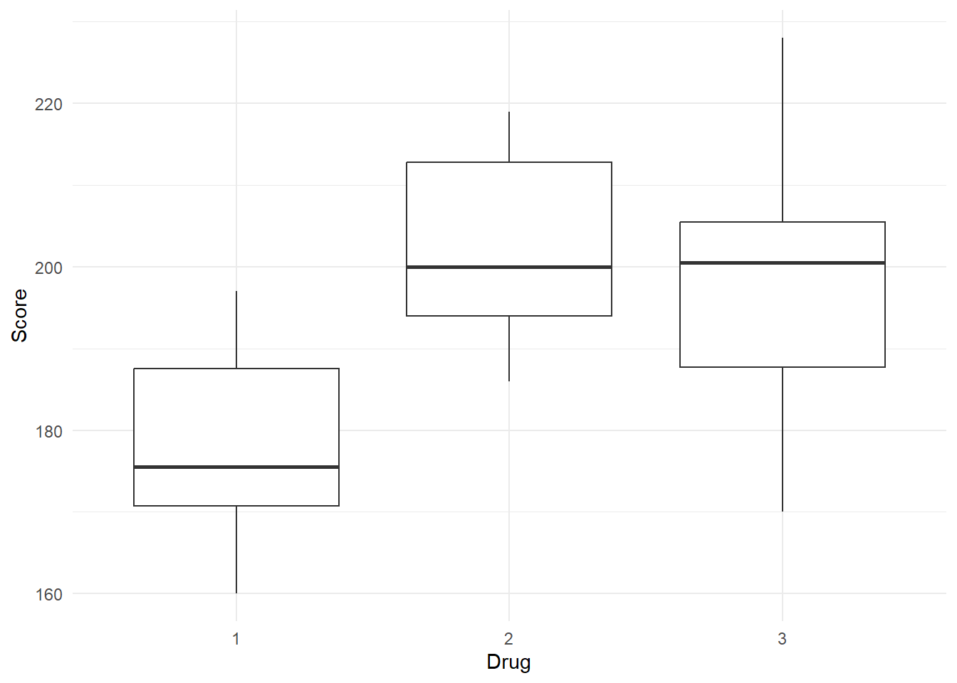

By Feedback

# Summary statistics
data %>% 
  group_by(Feedback) %>%
  summarise(
    n = n(),
    min = min(Score),
    max = max(Score),
    median = median(Score),
    mean = mean(Score),
    sd = sd(Score)   
    ) %>%
  gt::gt()

Feedback	n	min	max	median	mean	sd
1	15	160	219	186	187	17.96823
2	15	173	228	197	199	15.62507

data %>%
  ggplot(aes(x = Feedback, y = Score)) +
  geom_boxplot() +
  theme_minimal()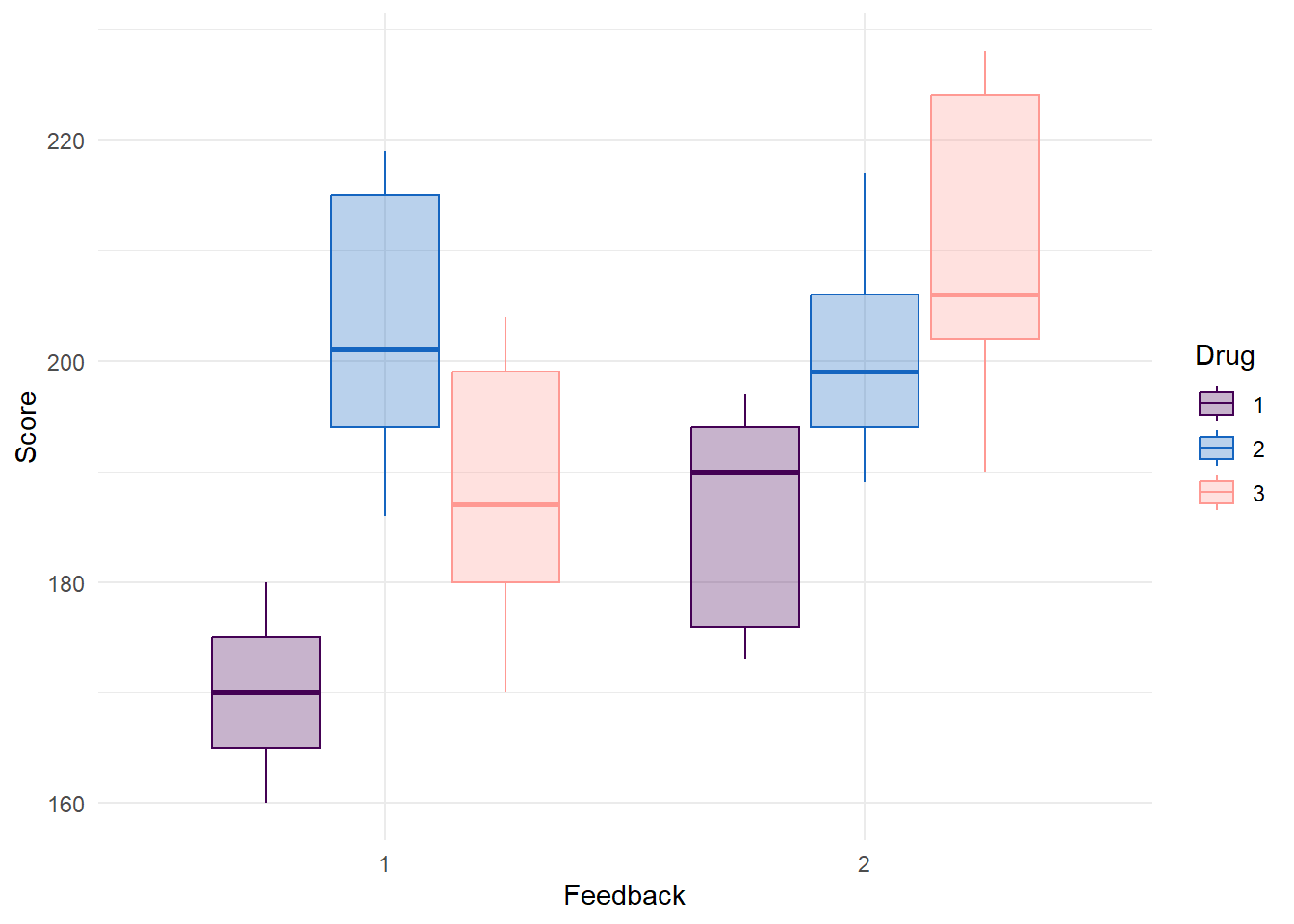

Plot Ddrug and Feedback

data %>%
  ggplot(aes(x = Feedback, y = Score, color = Drug, fill = Drug)) +
  geom_boxplot(alpha = 0.3) +
  scale_color_manual(values = c("#440154FF","#1565c0", "#FF9993")) +
  scale_fill_manual(values = c("#440154FF","#1565c0", "#FF9993")) +
  theme_minimal()

Summary statistics by Drug x Feedback (cell means)

# Summary statistics
summary_data <- data %>% 
  group_by(Feedback, Drug) %>%
  summarise(
    n = n(),
    min = min(Score),
    max = max(Score),
    median = median(Score),
    mean = mean(Score),
    sd = sd(Score),
    .groups = "drop"   
    ) 
    
summary_data %>%
  gt::gt()

Feedback	Drug	n	min	max	median	mean	sd
1	1	5	160	180	170	170	7.905694
1	2	5	186	219	201	203	13.910428
1	3	5	170	204	187	188	13.838353
2	1	5	173	197	190	186	10.839742
2	2	5	189	217	199	201	10.931606
2	3	5	190	228	206	210	15.811388

Perform the two-way ANOVA

To perform a two-way ANOVA in base R, we can use the same lm() function used in the one-way ANOVA and input the formula as an argument.

# Specify an lm() model
model <-  lm(Score ~ Feedback * Drug, data = data)

aov_tab <- car::Anova(model, type = "III")

# Print out the ANOVA table
aov_tab %>% 
  as.data.frame() %>%
  rownames_to_column(var = "Source") %>%
  gt::gt() %>%
  gt::fmt_number(
    columns = c("F value"),
    decimals = 2  # Use `decimals` for fixed decimal places
  ) %>%
  gt::fmt(
    columns = c("Pr(>F)"),
    fns = function(x) {
      ifelse(x < 0.001, "< 0.001", formatC(x, format = "f", digits = 3))
    }
  )

Source	Sum Sq	Df	F value	Pr(>F)
(Intercept)	144500	1	927.77	< 0.001
Feedback	640	1	4.11	0.054
Drug	2730	2	8.76	0.001
Feedback:Drug	780	2	2.50	0.103
Residuals	3738	24	NA	NA

Effect size

eta_squared <- effectsize::eta_squared(car::Anova(model, type = 3), partial = TRUE)  %>%
  gt::gt() %>%
  gt::fmt_number(
    columns = c("Eta2_partial", "CI_low"),
    decimals = 3  # Use `decimals` for fixed decimal places
  )

Interaction plot

ggplot(summary_data, aes(x = Feedback, y = mean, group = Drug, color = Drug)) +
  geom_line(linewidth = 1) +    # Connect means with lines
  geom_point(size = 3) +   # Add points for means
  scale_color_manual(values = c("#440154FF","#1565c0", "#FF9993")) +
  theme_minimal() +
  labs(y = "Mean BP")

Tests of estimated marginal means

Suppose we wanted to know the overall difference between Feedback and no Feedback. Or we wanted to know the difference between between Drug 1 and Drug 2. Tests of estimated marginal means would be one way to accomplish this. In SAS these are referred to as least squares means (LS means). In R we essentially create a contrast to compare two groups.

Feedback

# Test of marginal means for Feedback
pwc <- emmeans::emmeans(model, ~ Feedback) %>%
  pairs() %>%
  as_tibble() 
  
# Format the pwc table for display
pwc %>%
  gt::gt() %>%
  gt::fmt_number(
    columns = c("SE", "t.ratio"),
    decimals = 2  # Use `decimals` for fixed decimal places
  ) %>%
  gt::fmt(
    columns = c("p.value"),
    fns = function(x) {
      ifelse(x < 0.001, "< 0.001", formatC(x, format = "f", digits = 3))
    }
  )

contrast	estimate	SE	df	t.ratio	p.value
Feedback1 - Feedback2	-12	4.56	24	−2.63	0.015

emms <- emmeans::emmeans(model, ~ Feedback) %>%
  as_tibble()

NOTE: Results may be misleading due to involvement in interactions

# Print the estimated marginal means of Feedback
emms %>%
  gt::gt() %>%
  gt::fmt_number(
    columns = c("SE", "lower.CL", "upper.CL"),
    decimals = 2  # Use `decimals` for fixed decimal places
  )

Feedback	emmean	SE	df	lower.CL	upper.CL
1	187	3.22	24	180.35	193.65
2	199	3.22	24	192.35	205.65

# Plot the 
emms %>%
  ggplot(aes(x = Feedback, y = emmean)) +
  geom_point() +
  geom_errorbar(
    aes(ymin = lower.CL, ymax = upper.CL),
    width = 0.1) +
  theme_minimal()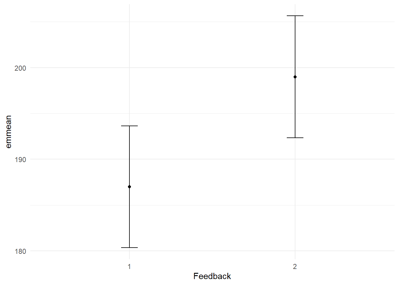

Drug

# Test of marginal means for Drug
pwc <- emmeans::emmeans(model, ~ Drug) %>%
  pairs() %>%
  as_tibble()
  
pwc %>%
  gt::gt() %>%
    gt::fmt_number(
    columns = c("SE", "t.ratio"),
    decimals = 2  # Use `decimals` for fixed decimal places
  ) %>%
  gt::fmt(
    columns = c("p.value"),
    fns = function(x) {
      ifelse(x < 0.001, "< 0.001", formatC(x, format = "f", digits = 3))
    }
  )

contrast	estimate	SE	df	t.ratio	p.value
Drug1 - Drug2	-24	5.58	24	−4.30	< 0.001
Drug1 - Drug3	-21	5.58	24	−3.76	0.003
Drug2 - Drug3	3	5.58	24	0.54	0.854

emms <- emmeans::emmeans(model, ~ Drug) %>%
  as_tibble() 

NOTE: Results may be misleading due to involvement in interactions

# Print the estimated marginal means of Drug
emms %>%
  gt::gt() %>%
  gt::fmt_number(
    columns = c("SE", "lower.CL", "upper.CL"),
    decimals = 2  # Use `decimals` for fixed decimal places
  )

Drug	emmean	SE	df	lower.CL	upper.CL
1	178	3.95	24	169.85	186.15
2	202	3.95	24	193.85	210.15
3	199	3.95	24	190.85	207.15

# Plot the means and the 95% CIs
emms %>%
  ggplot(aes(x = Drug, y = emmean)) +
  geom_point() +
  geom_errorbar(
    aes(ymin = lower.CL, ymax = upper.CL),
    width = 0.1) +
  theme_minimal()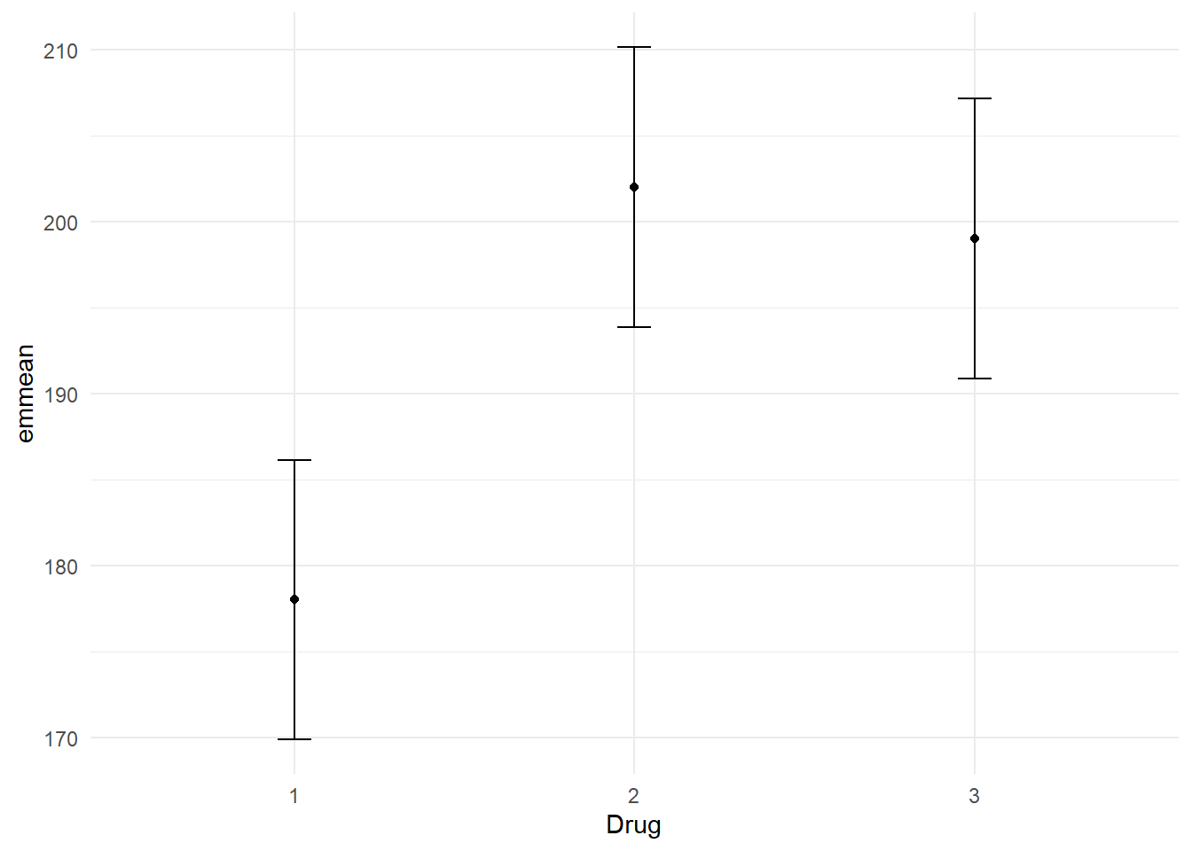

Interpretation

The omnibus Type III ANOVA revealed no significant interaction between Drug and Feedback, F(2, 24) = 2.50, p = .103, partial η² = .173. However, there were significant main effects. The main effect of Feedback was significant F(1, 24) = 6.93, p = .015, partial η² = .15. Post-hoc pairwise comparisons revealed an estimated reduction of 12 units in blood pressure with biofeedback, t = -2.63, p = 0.015, CI[3.062, 20.94]. Given the absence of a statistically significant interaction, we proceeded with tests of estimated marginal means to examine the main effects. The main effect of Drug was significant F(2, 24) = 10.98, p < .001, partial η² = .42. Post-hoc pairwise comparisons revealed an estimated reduction of 24 units in blood pressure for those on Drug 1 compared to Drug 2, t = -4.3, p < 0.001, CI[13.06, 34.94]. Similarly, those on Drug 1 had an estimated reduction of 21 units in blood pressure compared to those on Drug 3, t = -3.76, p = 0.003, CI[10.06, 31.94]. A comparison between Drug 2 and Drug 3 did not reveal a significant difference in blood pressure, t = 0.54, p = 0.854, CI[-13.94, 7.94].

If a significant interaction had been present, the appropriate next step would have been to test simple effects (e.g., Drug within levels of Feedback, or Fedback within levels of Drug). Nevertheless, the choice between marginal means and simple effects should ultimately be driven by the underlying research questions and theoretical considerations of the research question of interest.

References

Maxwell, Scott, Harold Delaney, and Ken Kelley. 2020. AMCP: A Model Comparison Perspective. https://CRAN.R-project.org/package=AMCP.

Maxwell, Scott E, Harold D Delaney, and Ken Kelley. 2017. Designing Experiments and Analyzing Data: A Model Comparison Perspective. Routledge.

Wickham, Hadley. 2019. Tidyverse: Easily Install and Load the ’Tidyverse’. https://CRAN.R-project.org/package=tidyverse.