library(tidyverse)
library(gtsummary)
library(dfmtbx)Generalized Linear Mixed Models: Longitudinal Ordinal Outcome
Dataset description
Generate summary statistics
Observed proportions
obs_props <- data %>%
  drop_na(tx) %>%
  filter(week %in% c(0, 1, 3, 6)) %>%
  mutate(week = str_c("Week", week)) %>%
  mutate(
    imps79o_1 = ifelse(imps79o == 1, 1, 0),
    imps79o_2 = ifelse(imps79o == 2, 1, 0),
    imps79o_3 = ifelse(imps79o == 3, 1, 0),
    imps79o_4 = ifelse(imps79o == 4, 1, 0)
  ) %>%
  group_by(tx, week) %>%
  summarise(
    p1 = mean(imps79o_1, na.rm = TRUE),
    p2 = mean(imps79o_2, na.rm = TRUE),
    p3 = mean(imps79o_3, na.rm = TRUE),
    p4 = mean(imps79o_4, na.rm = TRUE),
    .groups = "drop"
  ) %>%
  mutate(tx = ifelse(tx == 0, "Placebo", "Drug"))

obs_props %>%
   mutate(across(p1:p4, ~ as.character(round(.x, 3)))) %>%
format_gt_tbl()| tx | week | p1 | p2 | p3 | p4 |
|---|---|---|---|---|---|
| Placebo | Week0 | 0 | 0.103 | 0.336 | 0.561 |
| Placebo | Week1 | 0.019 | 0.238 | 0.248 | 0.495 |
| Placebo | Week3 | 0.034 | 0.276 | 0.299 | 0.391 |
| Placebo | Week6 | 0.114 | 0.343 | 0.229 | 0.314 |
| Drug | Week0 | 0.003 | 0.131 | 0.263 | 0.602 |
| Drug | Week1 | 0.065 | 0.343 | 0.305 | 0.287 |
| Drug | Week3 | 0.178 | 0.376 | 0.303 | 0.143 |
| Drug | Week6 | 0.351 | 0.445 | 0.125 | 0.079 |
Observed cumulative odds
# Calculate the odds for each group in weeks 0, 1, 3, and 6
obs_codds <- obs_props %>%
  mutate(
    codds1 = (p2 + p3 + p4) / p1,
    codds2 = (p3 + p4) / (p1 + p2),
    codds3 = p4 / (p1 + p2 + p3)
    ) %>%
  select(tx, week, codds1:codds3)

obs_codds %>%
  mutate(across(codds1:codds3, ~ as.character(round(.x, 3)))) %>%
format_gt_tbl()| tx | week | codds1 | codds2 | codds3 |
|---|---|---|---|---|
| Placebo | Week0 | Inf | 8.727 | 1.277 |
| Placebo | Week1 | 51.5 | 2.889 | 0.981 |
| Placebo | Week3 | 28 | 2.222 | 0.642 |
| Placebo | Week6 | 7.75 | 1.188 | 0.458 |
| Drug | Week0 | 326 | 6.432 | 1.515 |
| Drug | Week1 | 14.286 | 1.45 | 0.402 |
| Drug | Week3 | 4.627 | 0.805 | 0.167 |
| Drug | Week6 | 1.849 | 0.256 | 0.086 |
Observed log odds (logits)
# Calculate the log odds (logits)
obs_clogits <- obs_codds %>%
  mutate(across(-(tx:week), ~ log(.x))) %>%
  rename(
    clogit1 = codds1,
    clogit2 = codds2,
    clogit3 = codds3
  )

obs_clogits %>%
  mutate(across(clogit1:clogit3, ~ as.character(round(.x, 3)))) %>%
format_gt_tbl()| tx | week | clogit1 | clogit2 | clogit3 |
|---|---|---|---|---|
| Placebo | Week0 | Inf | 2.166 | 0.244 |
| Placebo | Week1 | 3.942 | 1.061 | -0.019 |
| Placebo | Week3 | 3.332 | 0.799 | -0.444 |
| Placebo | Week6 | 2.048 | 0.172 | -0.78 |
| Drug | Week0 | 5.787 | 1.861 | 0.416 |
| Drug | Week1 | 2.659 | 0.372 | -0.912 |
| Drug | Week3 | 1.532 | -0.217 | -1.792 |
| Drug | Week6 | 0.615 | -1.363 | -2.453 |
#|echo: false
# on the logit scale the reference is 0
# which means the probability is .5
# small differences in probability will get amplified in the odds
Visualize data
# Plot the cumulative logits (log(odds)) vs time in weeks
obs_clogits %>%
  pivot_longer(
    cols = -(tx:week),
    names_to = "logit",
    values_to = "clogit") %>%
  mutate(sweek = sqrt(as.numeric(substr(week, 5, 5)))) %>%
  filter(clogit != Inf) %>%
  ggplot(aes(x = sweek, y = clogit, color = tx, group = tx)) +
  geom_line() +
  geom_point() +
  # scale_x_continuous(breaks = c(0, seq(1:6))) +
  theme_minimal() +
  theme(legend.position = "bottom") +
  facet_wrap(~ logit)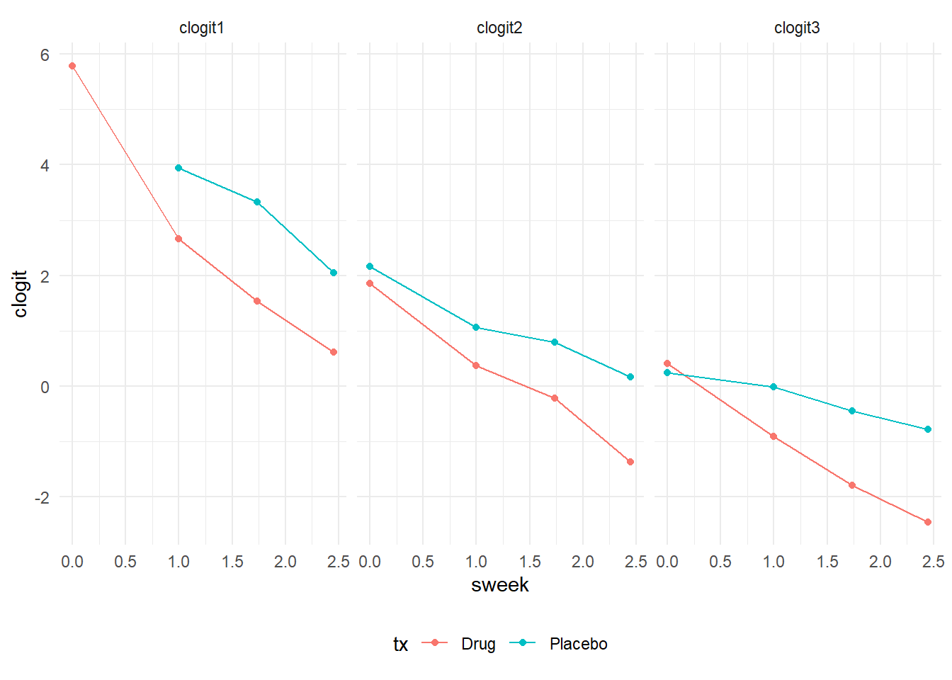
Random intercept model
data <- data %>%
  mutate(imps79o = factor(imps79o, levels = c(1,2,3,4)))

model_tab_10.2 <- ordinal::clmm(
  imps79o ~ tx * sweek + (1 | id),
  link = "logit",
  data = data,
  nAGQ = 7
)

summary(model_tab_10.2)
Cumulative Link Mixed Model fitted with the adaptive Gauss-Hermite
quadrature approximation with 7 quadrature points
formula: imps79o ~ tx * sweek + (1 | id)
data: data
link threshold nobs logLik AIC niter max.grad cond.H
logit flexible 1603 -1701.39 3416.78 467(2174) 1.90e-04 2.4e+02
Random effects:
Groups Name Variance Std.Dev.
id (Intercept) 3.772 1.942
Number of groups: id 437
Coefficients:
Estimate Std. Error z value Pr(>|z|)
tx -0.05852 0.31372 -0.187 0.852
sweek -0.76581 0.13077 -5.856 4.73e-09 ***
tx:sweek -1.20600 0.15266 -7.900 2.79e-15 ***
---
Signif. codes: 0 '***' 0.001 '**' 0.01 '*' 0.05 '.' 0.1 ' ' 1
Threshold coefficients:
Estimate Std. Error z value
1|2 -5.8590 0.3318 -17.657
2|3 -2.8263 0.2900 -9.746
3|4 -0.7085 0.2749 -2.577
(1456 observations deleted due to missingness)Random intercept and trend
model_tab_10.3 <- ordinal::clmm(
  imps79o ~ tx * sweek + (sweek | id),
  link = "logit",
  data = data,
  nAGQ = 1
)

summary(model_tab_10.3)
Cumulative Link Mixed Model fitted with the Laplace approximation
formula: imps79o ~ tx * sweek + (sweek | id)
data: data
link threshold nobs logLik AIC niter max.grad cond.H
logit flexible 1603 -1679.31 3376.62 906(5281) 9.60e-05 1.8e+02
Random effects:
Groups Name Variance Std.Dev. Corr
id (Intercept) 6.054 2.461
sweek 1.613 1.270 -0.352
Number of groups: id 437
Coefficients:
Estimate Std. Error z value Pr(>|z|)
tx 0.0382 0.3718 0.103 0.918
sweek -0.8593 0.2076 -4.139 3.49e-05 ***
tx:sweek -1.6572 0.2401 -6.902 5.12e-12 ***
---
Signif. codes: 0 '***' 0.001 '**' 0.01 '*' 0.05 '.' 0.1 ' ' 1
Threshold coefficients:
Estimate Std. Error z value
1|2 -7.1772 0.4730 -15.173
2|3 -3.3505 0.3786 -8.850
3|4 -0.8086 0.3372 -2.398
(1456 observations deleted due to missingness)get_5050_p <- function(chi_stat) {
# Chi-square on 1 df
p1 <- pchisq(chi_stat, 1, lower.tail = FALSE)
# Chi-square on 2 df
p2 <- pchisq(chi_stat, 2, lower.tail = FALSE)
# Calculate p value
p = .5 * (p1 + p2) # Alternatively (p1 / 2) + (p2 / 2)
print(
str_c("chi2: ", chi_stat, ", ", "p: = ", p)
)
}
get_5050_p((1362 - 1249.7))[1] "chi2: 112.3, p: = 2.21104416538189e-25"Intraclass correlation coefficient
var <- 2.12^2

icc <- var / (var + ((pi^2) / 3))

icc
[1] 0.5773696Interpretation
References
Hedeker, Donald; Gibbons, Robert D. (2006). Longitudinal Data Analysis. Wiley.
Hedeker, D., du Toit, S. H., Demirtas, H. and Gibbons, R. D. (2018), A note on marginalization of regression parameters from mixed models of binary outcomes. Biometrics 74, 354–361. doi:10.1111/biom.12707
Rizopoulos D (2025). GLMMadaptive: Generalized Linear Mixed Models using Adaptive Gaussian Quadrature. R package version 0.9-7, https://CRAN.R-project.org/package=GLMMadaptive.