Generalized Estimating Equations (GEE) for Longitudinal Binary Outcomes

library(tidyverse)
library(gtsummary)
library(dfmtbx)

Generalized estimating equations (GEE) are often described as an extension of generalized linear models for situations with correlated data. As a result, they are frequently used to analyze longitudinal data.

Although GEEs described as ext of glmms, they can be used for continuous outcomes.

GEE models can be used to analyze continuous, binary, count, and categorical longitudinal outcomes. In this respect, they are not much different than linear and generalized linear mixed models. The distinguishing feature about GEE models is their emphasis on marginal as opposed to conditional effects. Marginal effects are described as population-average effects. GEE models are well-suited for scientific questions regarding the average effect of a treatment in the population. In contrast, conditional or subject-specific effects are well-suited for research questions regarding how a treatment changes an individual’s trajectory, given their random effects.

In cases where the outcome is continuous and one clustering variable is specified, the fixed effects from a linear mixed model will match or be close to the fixed effects from a GEE model under an exchangeable correlation structure (more on this later). The standard errors will be different because the two models estimate uncertainty differently. The test statistics will also be different because lmerTest() uses t-tests with Satterthwaite’s degrees of freedom by default, whereas the geeglm() uses Wald tests. Nevertheless, the two models will produce comparable estimates.

model_tab_4.3 <- lmerTest::lmer(
  hamd ~ week + (1 | subject), 
  data = data, 
  REML = FALSE
)
broom.mixed::tidy(model_tab_4.3)

# A tibble: 4 × 8
  effect   group    term            estimate std.error statistic    df   p.value
  <chr>    <chr>    <chr>              <dbl>     <dbl>     <dbl> <dbl>     <dbl>
1 fixed    <NA>     (Intercept)        23.6      0.639      36.9  121.  8.84e-68
2 fixed    <NA>     week               -2.38     0.135     -17.6  311.  1.33e-48
3 ran_pars subject  sd__(Intercept)     4.02    NA          NA     NA  NA       
4 ran_pars Residual sd__Observation     4.36    NA          NA     NA  NA

gee_model <- geepack::geeglm(
  hamd ~ week,
  id = subject,
  data = data,
  family = gaussian,
  corstr = "exchangeable"
)

broom::tidy(gee_model)

# A tibble: 2 × 5
  term        estimate std.error statistic p.value
  <chr>          <dbl>     <dbl>     <dbl>   <dbl>
1 (Intercept)    23.6      0.541     1896.       0
2 week           -2.38     0.202      138.       0

Dataset description

data <- mice::toenail %>%
  rename(tx = treatment) %>%
  tibble()

data <- left_join(
  data,
  data %>%
    select(visit) %>%
    distinct() %>%
    mutate(visit_mo = c(0, 4, 8, 12, 24, 36, 48) / 4), # Convert weeks to months
  by = "visit"
)

head(data)

# A tibble: 6 × 6
     ID outcome    tx  month visit visit_mo
  <int>   <int> <int>  <dbl> <int>    <dbl>
1     1       1     1  0         1        0
2     1       1     1  0.857     2        1
3     1       1     1  3.54      3        2
4     1       0     1  4.54      4        3
5     1       0     1  7.54      5        6
6     1       0     1 10.0       6        9

Exploratory data analysis

# Number of non-missing values by visit and treatment group
data %>%
  mutate(tx = ifelse(tx == 0, "Itraconazole", "Terbinafine")) %>%
  group_by(tx) %>%
  summarize(
    N = sum(visit == 1),
    Visit1 = sum(!is.na(outcome) & visit == 1),
    Visit2 = sum(!is.na(outcome) & visit == 2),
    Visit3 = sum(!is.na(outcome) & visit == 3),
    Visit4 = sum(!is.na(outcome) & visit == 4),
    Visit5 = sum(!is.na(outcome) & visit == 5),
    Visit6 = sum(!is.na(outcome) & visit == 6),
    Visit6 = sum(!is.na(outcome) & visit == 7)
  ) %>%
  format_gt_tbl()

tx	N	Visit1	Visit2	Visit3	Visit4	Visit5	Visit6
Itraconazole	146	146	141	138	132	130	133
Terbinafine	148	148	147	145	140	133	131

Generate summary statistics

Observed proportions

# Tabulate the proportion of participants with moderate or severe oncholysis
prop_by_visit <- data %>%
  mutate(visit = str_c("Visit", visit)) %>%
  group_by(tx, visit) %>%
  summarise(
    prop = mean(outcome, na.rm = TRUE), .groups = "drop"
  ) %>%
  pivot_wider(
    names_from = visit,
    values_from = prop) %>%
  mutate(tx = ifelse(tx == 0, "Itraconazole", "Terbinafine")) %>%
  ungroup() 
  
prop_by_visit %>%
  format_gt_tbl()

Observed proportions of >= “severely ill”
tx	Visit1	Visit2	Visit3	Visit4	Visit5	Visit6	Visit7
Itraconazole	0.370	0.348	0.319	0.220	0.108	0.085	0.105
Terbinafine	0.372	0.327	0.276	0.207	0.060	0.063	0.046

Observed odds

# Calculate the odds for each group by visit
odds_by_visit <- data %>%
  group_by(tx, visit) %>%
  summarise(
    ill = sum(outcome, na.rm = TRUE),
    not_ill = sum(outcome == 0, na.rm = TRUE),
    .groups = "drop"
  ) %>%
  mutate(odds = ill / not_ill) %>%
  select(tx, visit, odds) %>%
  mutate(visit = str_c("Visit", visit)) %>%
  pivot_wider(names_from = visit, values_from = odds) %>%
  mutate(tx = ifelse(tx == 0, "Itraconazole", "Terbinafine"))

odds_by_visit %>%
  format_gt_tbl()

Observed odds of >= “severely ill”
tx	Visit1	Visit2	Visit3	Visit4	Visit5	Visit6	Visit7
Itraconazole	0.587	0.533	0.468	0.282	0.121	0.093	0.118
Terbinafine	0.591	0.485	0.381	0.261	0.064	0.067	0.048

Observed log odds (logits)

# Calculate the log odds (logits)
logits_by_visit <- odds_by_visit %>%
  mutate(across(-tx, ~ log(.x)))

logits_by_visit %>%
  format_gt_tbl()

Observed log odds (logits) of “severely ill”
tx	Visit1	Visit2	Visit3	Visit4	Visit5	Visit6	Visit7
Itraconazole	−0.53	−0.63	−0.76	−1.27	−2.11	−2.37	−2.14
Terbinafine	−0.53	−0.72	−0.97	−1.34	−2.75	−2.70	−3.04

Differences in logits and the exponentiated differences

# Differences in the log(odds) for each group in each week
logit_diffs_by_visit <- logits_by_visit %>%
  arrange(tx) %>%
  select(-tx) %>%
  summarise_all( ~ diff(.x))
  
# Exponentiated differences in log odds
ors_by_visit <- logit_diffs_by_visit %>%
  mutate(across(everything(), ~ exp(.x)))

# Bind rows and display
bind_rows(
  logit_diffs_by_visit,
  ors_by_visit) %>%
  mutate(value = c("diff", "exp(diff)")) %>%
  select(value, everything()) %>%
  format_gt_tbl()

Difference in logits bettween groups and the exponentiated difference
value	Visit1	Visit2	Visit3	Visit4	Visit5	Visit6	Visit7
diff	0.01	−0.09	−0.21	−0.07	−0.63	−0.33	−0.90
exp(diff)	1.01	0.91	0.81	0.93	0.53	0.72	0.41

Visualize data

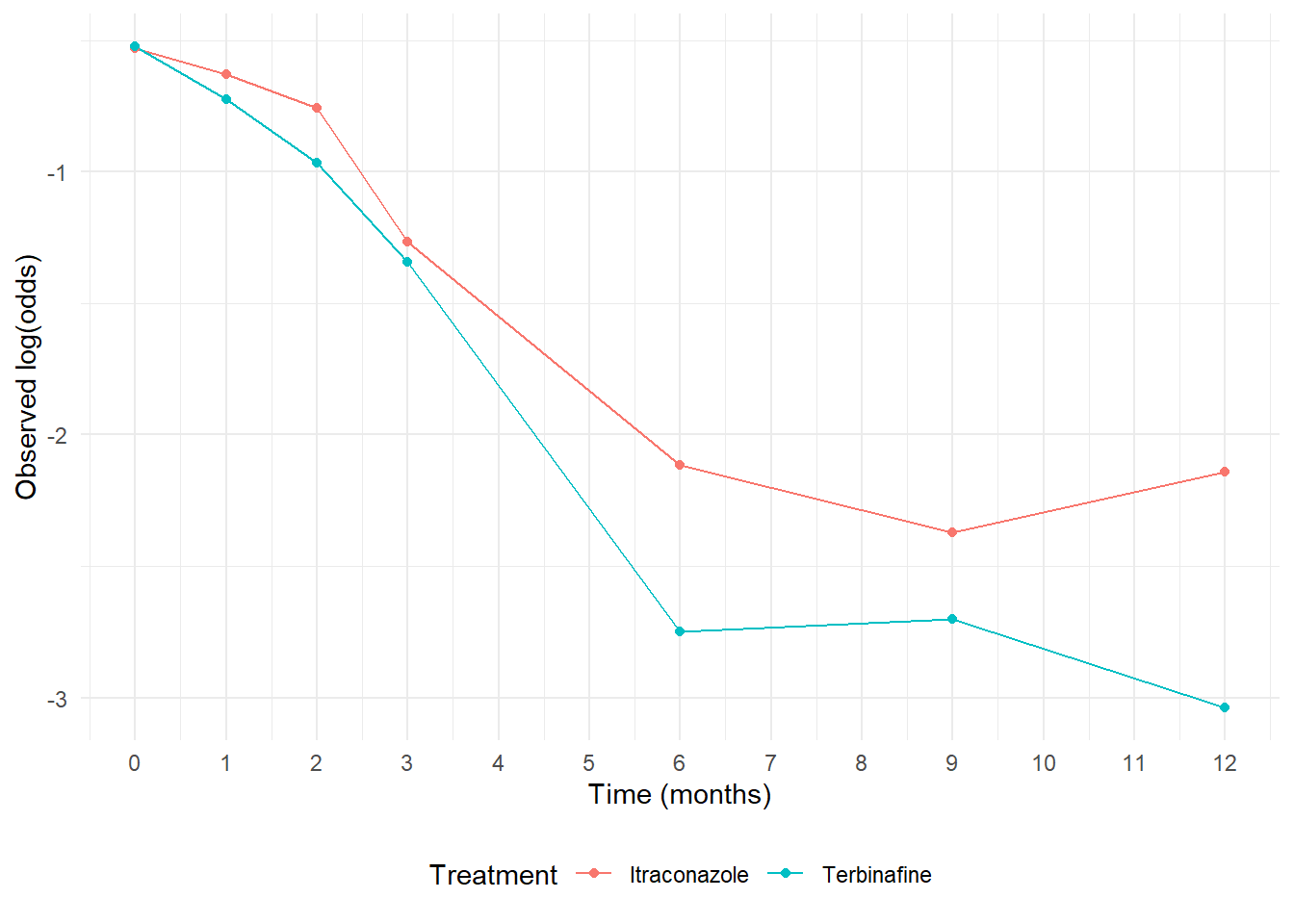
# Plot the logits (log(odds)) vs time
logits_by_visit %>%
  pivot_longer(cols = -tx, names_to = "week", values_to = "logit") %>%
  mutate(week = rep(c(0, 4, 8, 12, 24, 36, 48), 2)/4) %>%
  ggplot(aes(x = week, y = logit, color = tx, group = tx)) +
  geom_line() +
  geom_point() +
  scale_x_continuous(breaks = c(0, seq(1:13))) +
  theme_minimal() +
  labs(y = "Observed log(odds)", x = "Time (months)", color = "Treatment") +
  theme(legend.position = "bottom")

Missing data

GEE only valid if missing data are missing completely at random.

Data are only the observed rows.

data %>%
  group_by(ID) %>%
  count() %>%
  ungroup() %>%
  mutate(n_miss = 7 - n) %>%
  select(n_miss) %>%
  tbl_summary()

Characteristic	N = 294¹
n_miss
0	224 (76%)
1	39 (13%)
2	10 (3.4%)
3	6 (2.0%)
4	7 (2.4%)
5	3 (1.0%)
6	5 (1.7%)
¹ n (%)

# Create a long data set that includes the missing values ---------------------

# Convert the data to wide format
data_wide <- data %>%
  group_by(ID, tx) %>%
  select(ID, tx, visit, outcome) %>%
  pivot_wider(names_from = visit, values_from = outcome) %>%
  ungroup()

# Convert back to long to expose the missing values
data_long <- data_wide %>%
  group_by(ID) %>%
  pivot_longer(cols = c(`1`:`7`), values_to = "outcome", names_to = "visit") %>%
  ungroup()

# Merge in visit_mo
data_long <- data_long %>%
  mutate(visit = as.numeric(visit)) %>%
  left_join(data %>% select(visit, visit_mo) %>% distinct(), by = "visit")

# MCAR
# 1) define a missingness indicator "R"
data_long <- data_long %>%
  mutate(R = ifelse(is.na(outcome), 0, 1))

# 2) define lagged outcome
data_long <- data_long %>%
  arrange(ID, visit) %>%
  group_by(ID) %>%
  mutate(Y_lag = lag(outcome)) %>%
  ungroup()

# 3) fit a model using the missingness indicator as the outcome along with the 
# time, treatment, and lagged outcome variables as predictors
fit_miss <- glm(R ~ visit + tx + Y_lag,
                data = data_long,
                family = binomial)

summary(fit_miss)


Call:
glm(formula = R ~ visit + tx + Y_lag, family = binomial, data = data_long)

Coefficients:
            Estimate Std. Error z value Pr(>|z|)    
(Intercept)  3.94103    0.42380   9.299  < 2e-16 ***
visit       -0.21018    0.07465  -2.816  0.00487 ** 
tx           0.24336    0.23814   1.022  0.30683    
Y_lag       -0.17091    0.29612  -0.577  0.56384    
---
Signif. codes:  0 '***' 0.001 '**' 0.01 '*' 0.05 '.' 0.1 ' ' 1

(Dispersion parameter for binomial family taken to be 1)

    Null deviance: 609.64  on 1643  degrees of freedom
Residual deviance: 600.35  on 1640  degrees of freedom
  (414 observations deleted due to missingness)
AIC: 608.35

Number of Fisher Scoring iterations: 6

# naniar::mcar_test(data_long %>% select(ID, outcome, tx, visit))

Marginal effects model

# Marginal effects logistic regression model-----------------------------------
# There are options. use visit as fixed, month as continuous, convert weeks to months
# default corr structure is ind
model <- geepack::geeglm(
  outcome ~ tx*visit_mo,
  id = ID,
  family = "binomial",
  data = data
)

broom::tidy(model, conf.int = TRUE) %>%
  format_gt_tbl()

term	estimate	std.error	statistic	p.value	conf.low	conf.high
(Intercept)	−0.56	0.171	10.57	0.001	−0.89	−0.22
tx	0.02	0.251	0.01	0.924	−0.47	0.52
visit_mo	−0.18	0.030	34.39	< 0.001	−0.24	−0.12
tx:visit_mo	−0.08	0.055	2.06	0.151	−0.19	0.03

Trends and CIs

em <- emmeans::emtrends(model, ~ tx, var = "visit_mo")

em %>%
  as_tibble() %>%
  mutate(tx = ifelse(tx == 0, "Itraconazole", "Terbinafine")) %>%
  format_gt_tbl()

tx	visit_mo.trend	SE	df	lower.CL	upper.CL
Itraconazole	−0.18	0.030	1904	−0.24	−0.12
Terbinafine	−0.26	0.046	1904	−0.34	−0.17

Interpretation

The coefficient for the (Intercept) represents the predicted log odds of oncholysis in the Itraconazole group at baseline when the time variable is equal to 0.
The treatment main effect is 0.02. This represents the difference in odds of oncholysis in the Terbinafine group compared to Itraconazole at baseline. The coefficient, 0.02, is approximately equal to 1.02 when exponentiated. This suggests that the odds of oncholysis are 2% higher in the drug group compared to the Terbinafine group while holding time constant. However, this effect is not statistically significant.
The time main effect is -0.18. This coefficient represents the change in odds of oncholysis for each 1-unit increase in time for the Itraconazole group. The exponentiated coefficient is approximately equal to 0.84 and suggests that each 1-unit increase in time is associated with a 16% decrease in the odds of oncholysis. This effect is statisitically significant and suggests improvement in the odds of oncholysis over time.
The interaction effect is -0.08. This coefficient represents how the time slope in the Terbinafine group differs from the Itraconazole group. The exponentiated coefficient is approximately equal to 0.92 and suggests that the effect of time in the Terbinafine group is 8% lower than that of the Itraconazole group. -0.18 + (-0.08) = -0.26. The exponentiated value of -0.26 is approximately 0.77. This suggests that each 1-unit increase in time is associated with a 23% decrease in the odds of oncholysis in the Terbinafine group. However, this effect is not statistically significant.

# We summarize the inferential results using GEE below: reference is Itracanazole
# • Among those assigned to Itraconazole, the odds of severe infection is estimated to be 16% ((1- exp(-.18)) * 100)  (95% CI: 21% lower to 11% lower) per month.


# • Among those assigned to Terbinafine, the odds of severe infection is estimated to be 23% ((1- exp(-.18 + -0.08)) * 100) lower (95% CI: 29% lower to 15% lower) per month.


# • We do not have evidence that the ratio of odds of severe infection over time differs between the two
# groups (p = 0.151).