Welch's one-way ANOVA
When the homogeneity of variance assumption is violated for a one-way ANOVA, a Welch’s ANOVA can be conducted instead. One limitation for the Welch’s ANOVA is that it is restricted to data with only one explanatory factor (i.e. one-way between-subjects designs). This guide covers how to test for normality, homogeneity of variance and how to conduct a Welch’s ANOVA followed by the appropriate post hoc tests with the jmv and rstatix packages. The same example data from the one-way ANOVA are used here.
Perform ANOVA tests
The following code chunk demonstrates how to code a Welch’s ANOVA in R with the jmv package. The jmv approach uses the anovaOneW() function which can take options to produce plots and conduct tests of normality and equality of variance (homogeneity of variance or homoscedasticity) with the norm = TRUE and eqv = TRUE options respectively. Games-Howell post hoc tests are produced by setting phMethod = 'gamesHowell'.
library(jmv)
# Conduct Welch's ANOVA
anovaOneW(formula = Scores ~ Group,
          data = C3E9,
          welchs = TRUE,
          norm = TRUE,
          eqv = TRUE,
          phMethod = 'gamesHowell')
##
##  ONE-WAY ANOVA
##
##  One-Way ANOVA (Welch's)
##  ──────────────────────────────────────────────────────
##              F           df1    df2         p
##  ──────────────────────────────────────────────────────
##    Scores    7.692308      3    4.444444    0.0319410
##  ──────────────────────────────────────────────────────
##
##
##  ASSUMPTION CHECKS
##
##  Normality Test (Shapiro-Wilk)
##  ────────────────────────────────────
##              W            p
##  ────────────────────────────────────
##    Scores    0.8107880    0.0124591
##  ────────────────────────────────────
##    Note. A low p-value suggests a
##    violation of the assumption of
##    normality
##
##
##  Homogeneity of Variances Test (Levene's)
##  ─────────────────────────────────────────────────────
##              F               df1    df2    p
##  ─────────────────────────────────────────────────────
##    Scores    6.933348e-33      3      8    1.0000000
##  ─────────────────────────────────────────────────────
##
##
##  POST HOC TESTS
##
##  Games-Howell Post-Hoc Test – Scores
##  ────────────────────────────────────────────────────────────────────────────
##                            1            2            3            4
##  ────────────────────────────────────────────────────────────────────────────
##    1    Mean difference            —    -8.000000    -2.000000    -6.000000
##         p-value                    —    0.0270378    0.6456622    0.0689900
##
##    2    Mean difference                         —     6.000000     2.000000
##         p-value                                 —    0.0689900    0.6456622
##
##    3    Mean difference                                      —    -4.000000
##         p-value                                              —    0.2086312
##
##    4    Mean difference                                                   —
##         p-value                                                           —
##  ────────────────────────────────────────────────────────────────────────────
In rstatix, the anova_test() function can analyse several types of between and within subjects ANOVA designs. However, to conduct a Welch’s ANOVA , the welch_anova_test() function is required. The syntax to conduct the actual test is rather simple. In the following code chunk, I’ve chosen to explicitly declare formula = Scores ~ Group and data = C3E9. However, one could just as easily specify the dataframe and formula as long as data is the first entered variable. Similarly, data and formula do not need to be explicitly specified for the games_howell_test() function, but hare specified in the example for consistency.
Check normality
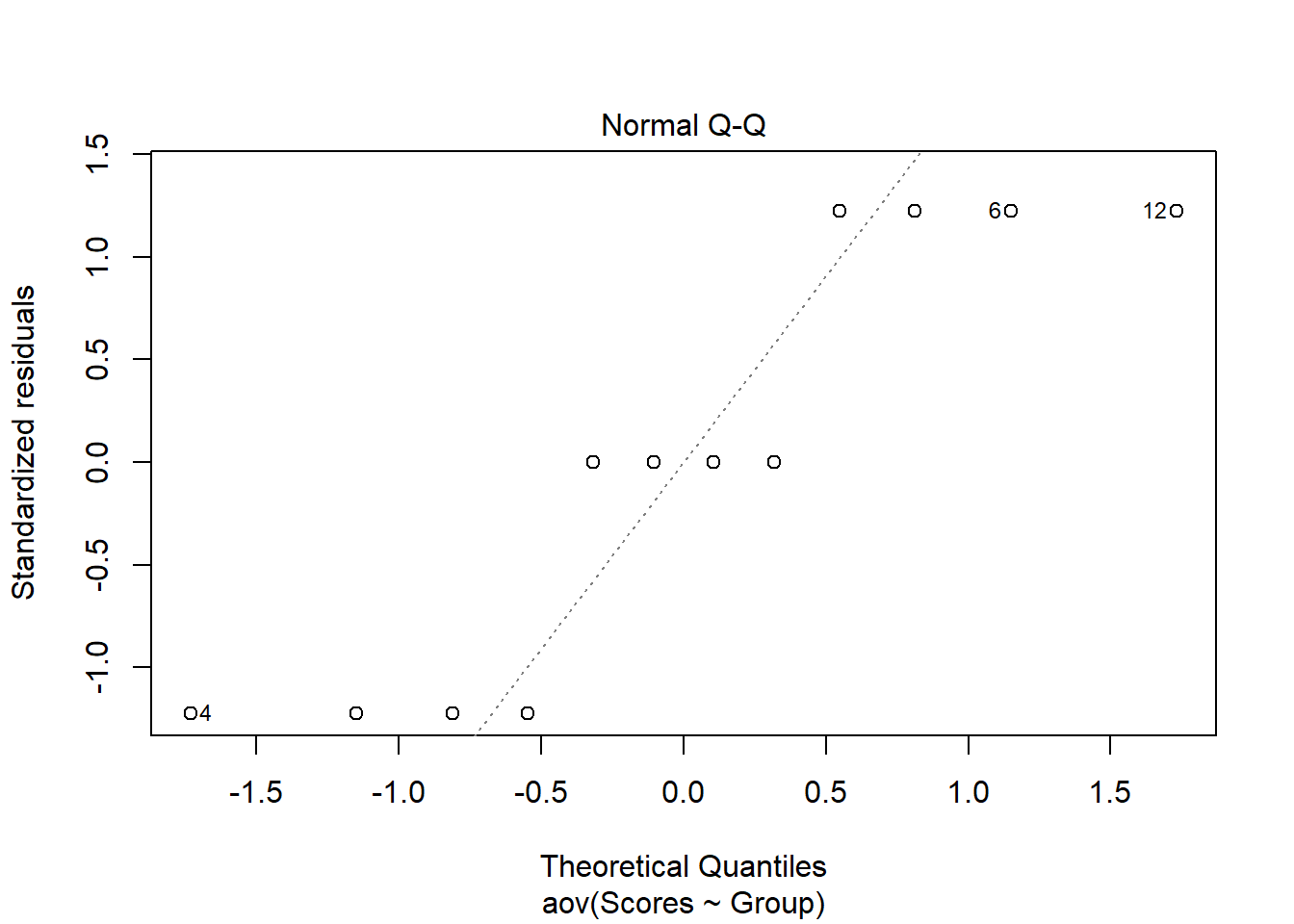
To produce the Shapiro-Wilk’s test of normality as in the jmv output, we will need to create an analysis of variance (aov) object with the base R aov() function. The aov() function is actually a wrapper for the lm() which highlights the relationship between linear regression and ANOVA. The rstatix package does contain its own shapiro_test() function, but it will not test normality of the residuals, only the actual values. In the code chunk below, the aov object is piped to the residuals() function, which is then piped to the shapiro.test() function. This will conduct Shapiro-Wilk’s test on the residuals of the aov object and not the values of the dependent variable. Our Shaprio-Wilk’s test result, W = 0.81 is significant with a p-values less than 0.05 which is taken as evidence that our data violate the assumption of normality.
In addition to the Shapiro-Wilk test, we can visualize the residuals of our data and plot them against the expected residuals of a normal distribution. If our data are normally distributed, we would expect the individual data points to hover near the diagonal line. As we can see in the plot, we have quite a few data points fall far away from the line which is additional evidence that our data are not normally distributed. When normality is violated, the Welch’s ANOVA is one option to analyse the data.
# Convert group to factor
C3E9$Group <- as.factor(C3E9$Group)

# Base R Shapiro-Wilk test on residuals of the aov object
aov(Scores ~ Group, data = C3E9) %>%
  residuals() %>%
  shapiro.test()
##
## 	Shapiro-Wilk normality test
##
## data:  .
## W = 0.81079, p-value = 0.01246
# Create a plot of standardised residuals, indexed at position 2 of plot(aov(x))
plot(aov(formula = Scores ~ Group, data = C3E9), 2)

Figure 1: Q-Q Plot
Check homogeneity of variance
Finally, for the homogeneity of variance test, the rstatix levene_test() function specifying a formula and a data frame does the job. The result is a non-significant p-value for the test statistic. This indicates that the data meet the assumption of homogeneity of variance.
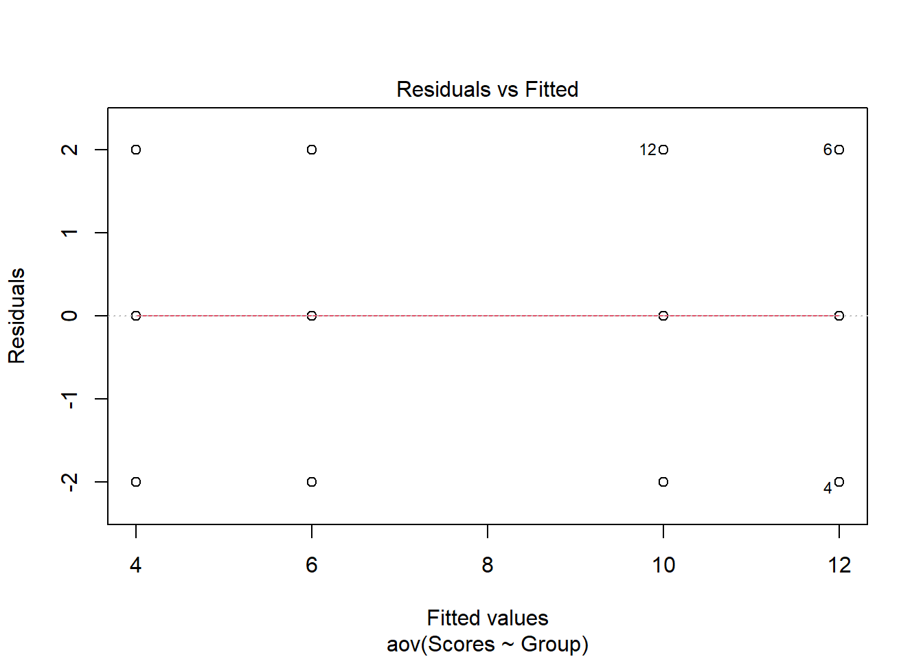
As in the examination of normality above, base R also can also plot the Residuals vs Fitted values to examine homogeneity of variance. The plot maintains a straight red line which is what would be expected for data that meet the homogeneity of variance assumption. When the assumption of homogeneity of variance is violated one can explore the use of a robust ANOVA.
library(rstatix)

# Residuals vs Fitted values plot
plot(aov(formula = Scores ~ Group, data = C3E9), 1)

Figure 2: Residuals vs Fitted Values
# rstatix Levene's test for homogeneity of variance
levene_test(formula = Scores ~ Group,
            data = C3E9)
## # A tibble: 1 × 4
##     df1   df2 statistic     p
##   <int> <int>     <dbl> <dbl>
## 1     3     8  6.93e-33     1
Welch’s ANOVA
Considering that the data failed to meet the assumption of normality, but met the assumption of homogeneity of variance, we can proceed to conduct a Welch’s ANOVA.
# Conduct Welch's ANOVA
welch_anova_test(formula = Scores ~ Group,
                 data = C3E9)
## # A tibble: 1 × 7
##   .y.        n statistic   DFn   DFd     p method
## * <chr>  <int>     <dbl> <dbl> <dbl> <dbl> <chr>
## 1 Scores    12      7.69     3  4.44 0.032 Welch ANOVA
# Alternatively
# welch_anova_test(C3E9, Scores ~ Group)
Post hoc tests
# Games-Howell post-hoc tests
games_howell_test(formula = Scores ~ Group,
                  data = C3E9,
                  conf.level = 0.95,
                  detailed = FALSE)
| .y. | group1 | group2 | estimate | conf.low | conf.high | p.adj | p.adj.signif |
|---|---|---|---|---|---|---|---|
| Scores | 1 | 2 | 8 | 1.3523215 | 14.6476785 | 0.027 | * |
| Scores | 1 | 3 | 2 | -4.6476785 | 8.6476785 | 0.646 | ns |
| Scores | 1 | 4 | 6 | -0.6476785 | 12.6476785 | 0.069 | ns |
| Scores | 2 | 3 | -6 | -12.6476785 | 0.6476785 | 0.069 | ns |
| Scores | 2 | 4 | -2 | -8.6476785 | 4.6476785 | 0.646 | ns |
| Scores | 3 | 4 | 4 | -2.6476785 | 10.6476785 | 0.209 | ns |
Interpretation
Both approaches produce the same results — a significant effect of the omnibus test [F(3, 4.44) = 7.69, p < 0.05]. Furthermore, Games-Howell post-hoc tests reveal a significant difference between the scores of group 1 (rational-emotive therapy) and group 2 (psychoanalytic therapy) with group 1 demonstrating lower mean phobia scores.
Wrap up
Similar to the one-way ANOVA guide, the anovaOneW() function from the jmv package is a convenient way to perform Welch’s one-way ANOVA in R. You can get a significant amount of output including normality, homogeneity of variance, and post-hoc tests by adding a few extra arguments to the call. To produce the same output with the rstatix package a little more work is necessary, but the results will be same.
References
Kassambara, Alboukadel. 2020a. Ggpubr: ’Ggplot2’ Based Publication Ready Plots. https://CRAN.R-project.org/package=ggpubr.
———. 2020b. Rstatix: Pipe-Friendly Framework for Basic Statistical Tests. https://CRAN.R-project.org/package=rstatix.
Maxwell, Scott, Harold Delaney, and Ken Kelley. 2020. AMCP: A Model Comparison Perspective. https://CRAN.R-project.org/package=AMCP.
Maxwell, Scott E, Harold D Delaney, and Ken Kelley. 2017. Designing Experiments and Analyzing Data: A Model Comparison Perspective. Routledge.
Selker, Ravi, Jonathon Love, and Damian Dropmann. 2020. Jmv: The ’Jamovi’ Analyses. https://CRAN.R-project.org/package=jmv.
Wickham, Hadley. 2019. Tidyverse: Easily Install and Load the ’Tidyverse’. https://CRAN.R-project.org/package=tidyverse.