Two-way ANOVA
This guide covers different ways of conducting two-way ANOVAs in R. Two-way ANOVAS are an extension of one-ways ANOVAS where an additional between-subjects factor is of interest.
The data set
The example data set comes from chapter_7_table_5 from the AMCP package. In the example data set, a hypothetical experiment tests the effect of presence or absence of biofeedback (first between-subjects factor) in combination with three different drugs on measures of blood pressure (second between-subjects ). The Feedback group is coded as a 1 or a 2 where 1 indicates the participants received biofeedback and 2 indicates participants did not. Drug is coded as 1, 2, or 3, and specifies one of three hypothetical drugs that purportedly reduce blood pressure. Finally, Scores refer to the dependent variable and measure blood pressure where lower values are better. This leaves us with a 2x3 between-subjects design. We will also assume that the assumptions of independence, equality of variance, and normality are met for the sample data set.
library(AMCP)

# Load data
data("chapter_7_table_5")

# Inspect data
kableExtra::kable(head(chapter_7_table_5))
| Score | Feedback | Drug |
|---|---|---|
| 170 | 1 | 1 |
| 175 | 1 | 1 |
| 165 | 1 | 1 |
| 180 | 1 | 1 |
| 160 | 1 | 1 |
| 186 | 1 | 2 |
Perform ANOVA tests
First, load the jmv package and use the ANOVA() function which can be used for both one-way and two-way designs. The following code will set Score as the dependent variable and Feedback and Drug as independent variables (between-subjects factors). The call is set to use type III sums of squares, the effect size for the omnibus test will be reported as partial eta squared, post hoc tests will be performed with Feedback and Drug factors, and the plots of the means of Feedback and Drug will be generated.
library(jmv)

# ANOVA test with jmv
ANOVA(formula = Score ~ Feedback * Drug,
      data = chapter_7_table_5,
      ss = "3",
      effectSize = 'partEta',
      postHoc = c('Feedback', 'Drug'),
      postHocCorr = 'none',
      postHocES = "d",
      emMeans = ~ Feedback + Drug,
      #emMeans = list(c("Feedback", "Drug")), #generates interaction plot
      emmPlots = TRUE,
      emmTables = TRUE,
      ciWidthEmm = 95)
##
##  ANOVA
##
##  ANOVA - Score
##  ───────────────────────────────────────────────────────────────────────────────────────────────
##                     Sum of Squares    df    Mean Square    F            p            η²p
##  ───────────────────────────────────────────────────────────────────────────────────────────────
##    Feedback              1080.0000     1      1080.0000     6.934189    0.0145635    0.2241594
##    Drug                  3420.0000     2      1710.0000    10.979133    0.0004113    0.4777871
##    Feedback:Drug          780.0000     2       390.0000     2.504013    0.1028767    0.1726428
##    Residuals             3738.0000    24       155.7500
##  ───────────────────────────────────────────────────────────────────────────────────────────────
##
##
##  POST HOC TESTS
##
##  Post Hoc Comparisons - Feedback
##  ────────────────────────────────────────────────────────────────────────────────────────────────────────────────
##    Feedback         Feedback    Mean Difference    SE          df          t            p            Cohen's d
##  ────────────────────────────────────────────────────────────────────────────────────────────────────────────────
##    1           -    2                 -12.00000    4.557046    24.00000    -2.633285    0.0145635    -0.9615397
##  ────────────────────────────────────────────────────────────────────────────────────────────────────────────────
##    Note. Comparisons are based on estimated marginal means
##
##
##  Post Hoc Comparisons - Drug
##  ─────────────────────────────────────────────────────────────────────────────────────────────────────────
##    Drug         Drug    Mean Difference    SE          df          t             p            Cohen's d
##  ─────────────────────────────────────────────────────────────────────────────────────────────────────────
##    1       -    2            -24.000000    5.581219    24.00000    -4.3001362    0.0002462    -1.9230794
##            -    3            -21.000000    5.581219    24.00000    -3.7626192    0.0009578    -1.6826945
##    2       -    3              3.000000    5.581219    24.00000     0.5375170    0.5958599     0.2403849
##  ─────────────────────────────────────────────────────────────────────────────────────────────────────────
##    Note. Comparisons are based on estimated marginal means
##
##
##  ESTIMATED MARGINAL MEANS
##
##  FEEDBACK
##
##  Estimated Marginal Means - Feedback
##  ────────────────────────────────────────────────────────────
##    Feedback    Mean        SE          Lower       Upper
##  ────────────────────────────────────────────────────────────
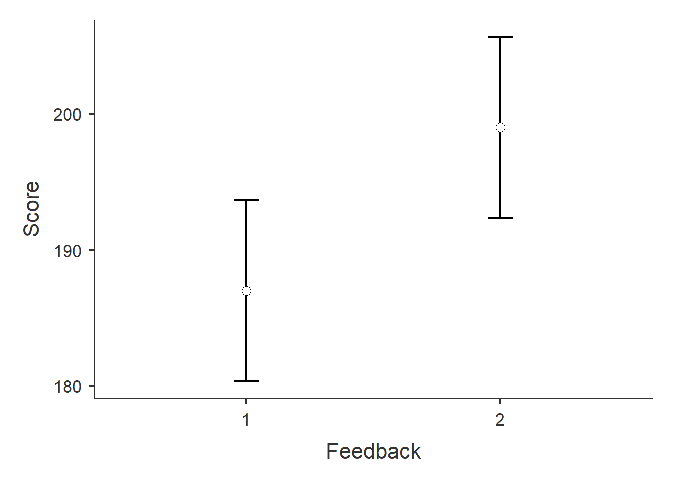
##    1           187.0000    3.222318    180.3495    193.6505
##    2           199.0000    3.222318    192.3495    205.6505
##  ────────────────────────────────────────────────────────────
##
##
##  DRUG
##
##  Estimated Marginal Means - Drug
##  ────────────────────────────────────────────────────────
##    Drug    Mean        SE          Lower       Upper
##  ────────────────────────────────────────────────────────
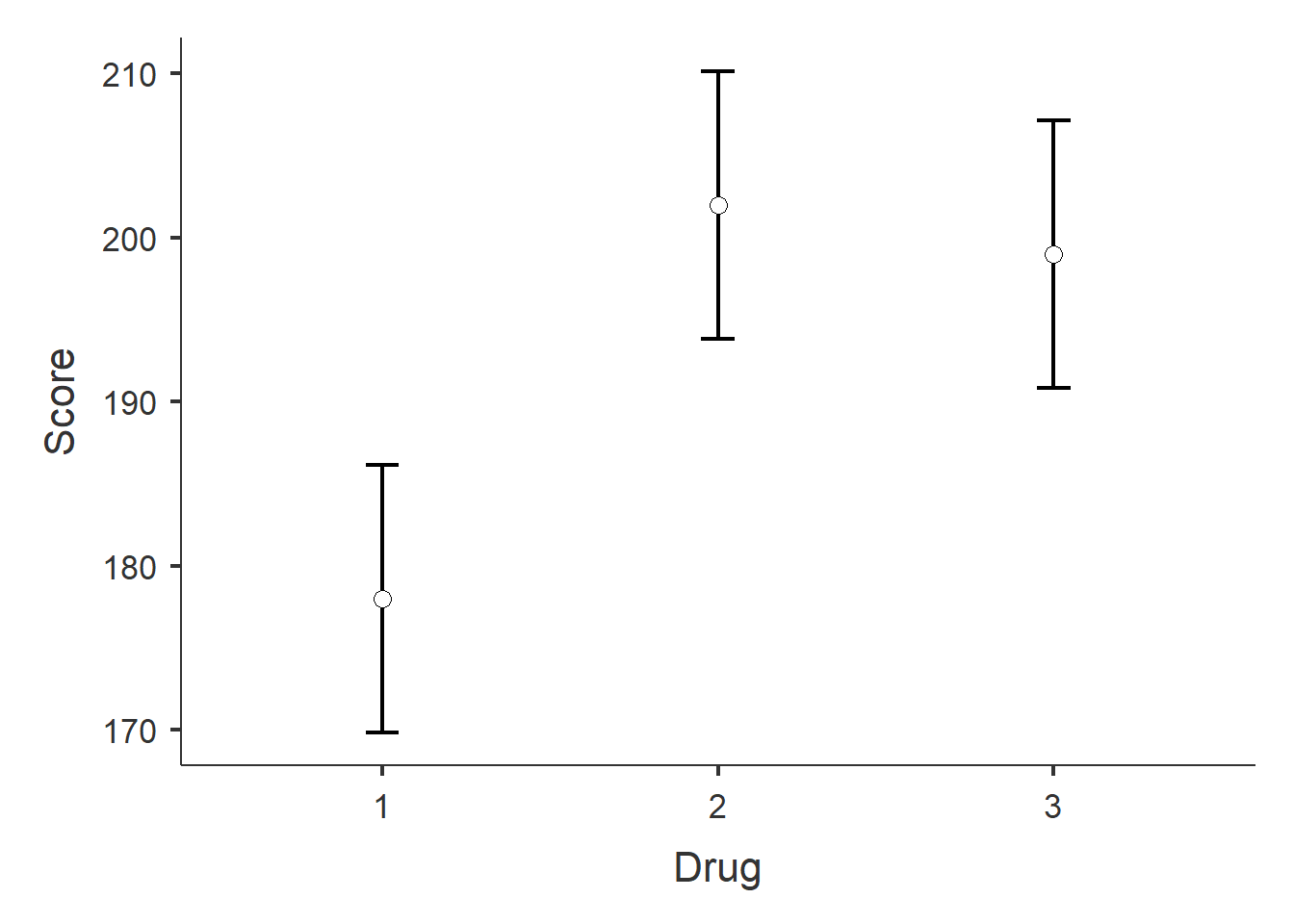
##    1       178.0000    3.946517    169.8548    186.1452
##    2       202.0000    3.946517    193.8548    210.1452
##    3       199.0000    3.946517    190.8548    207.1452
##  ────────────────────────────────────────────────────────

Figure 1: Estimated marginal means and confidence intervals.

Figure 2: Estimated marginal means and confidence intervals.
To perform a two-way ANOVA with the rstatix package, the Feedback and Drug variables first need to be converted to factor so the numerical values get treated as a categorical variable. Next, the anova_test() function can be used to conduct the test and display the results. However, it may be advantageous to first fit an aov() model that can later be used with the emmeans_test() function.
library(tidyverse)
library(rstatix)
library(ggpubr)

# Convert Drug and Feedback to factor
chapter_7_table_5 <- chapter_7_table_5 %>%
  mutate_at(c("Drug", "Feedback"), as.factor)

# Create aov() model
model <- aov(formula = Score ~ Feedback * Drug,
    data = chapter_7_table_5)

# anova_test on  model, with partial eta squared and type III ss
anova_test(model, effect.size = "pes", type = 3)
## ANOVA Table (type III tests)
##
##          Effect DFn DFd      F        p p<.05   pes
## 1      Feedback   1  24  6.934 0.015000     * 0.224
## 2          Drug   2  24 10.979 0.000411     * 0.478
## 3 Feedback:Drug   2  24  2.504 0.103000       0.173
# Alternative form of using anova_test()
# anova_test(Score ~ Feedback * Drug,
#            data = chapter_7_table_5,
#            effect.size = "pes",
#            type = 3)
The results from the omnibus test reveal that there is no significant interaction between Drug and Feedback. On the other hand, there are significant main effects for Drug and for Feedback. Because the interaction is not significant, we may proceed to perform tests of marginal means. Had the interaction been significant, we could have opted to perform tests of simple effects of Drug within Feedback, or Feedback within drug. However, these are primarily suggestions and the approach to analyzing the data should be guided by the research question.
Tests of marginal means
The rstatix package includes a function, emmeans_test(), that can perform tests of estimated marginal means. To perform these tests, we will use the aov model that we created in the previous step and we will conduct two separate tests, one for Feedback and one for Drug. The correction method in this example is set to "none", but this can be easily changed according to your situation. The available correction methods can be found by typing help(anova_test) in the Console.
We will also use the get_summary_stats() function and illustrate how the tidyverse package meshes with rstatix to produce descriptive statistics to aid in the interpretation of the output. First we will start with the chapter_7_table_5 data and pipe it to the group_by() function which will create subsets of data according to combinations of Drug and Feedback, then that output is fed into the get_summary_stats() which will calculate several descriptive statistics for each group. Finally, to display only a part of this output, the select() function will display data by specifying column names.
To plot the data we will rely on the ggpubr package. The ggpubr and rstatix packages are developed by the same individual and are aimed at simplifying the syntax for conducting statistical tests and generating plots in R. For our purposes we will use the ggerrorplot() function to plot means and confidence intervals.
Feedback
# Test of marginal means for Feedback
pwc <- chapter_7_table_5 %>%
  emmeans_test(Score ~ Feedback,
               p.adjust.method = "none",
               model = model)
## NOTE: Results may be misleading due to involvement in interactions
| term | .y. | group1 | group2 | df | statistic | p | p.adj | p.adj.signif |
|---|---|---|---|---|---|---|---|---|
| Feedback | Score | 1 | 2 | 24 | -2.633285 | 0.0145635 | 0.0145635 | * |
# Print the estimated marginal means of Feedback
get_emmeans(pwc) %>% kableExtra::kable(., "html")
| Feedback | emmean | se | df | conf.low | conf.high | method |
|---|---|---|---|---|---|---|
| 1 | 187 | 3.222318 | 24 | 180.3495 | 193.6505 | Emmeans test |
| 2 | 199 | 3.222318 | 24 | 192.3495 | 205.6505 | Emmeans test |
# Modify pwc to include x and y positions for plotting signficance markers
pwc <- pwc %>% add_xy_position(x = "Feedback", fun = "mean_ci")

# Generate an error plot uses ggpubr AND ggplot functions to layer the plot
ggerrorplot(get_emmeans(pwc),
       x = "Feedback",
       y = "emmean",
       ylab = "Mean BP Scores") +
    geom_errorbar(aes(ymin = conf.low, ymax = conf.high),
                  width = 0.1) +
    stat_pvalue_manual(pwc, hide.ns = TRUE, tip.length = FALSE)

Plot cell means
#Produce an error plot with cell means and ci instead of estimated marginal means
#The same code chunk can be used to get cell means of Drug by changing the "x = " argument
ggerrorplot(chapter_7_table_5,
       x = "Feedback",
       y = "Score",
       add = "mean",
       desc_stat = "mean_ci",
       error.plot = "errorbar",
       width = .1)

#Print cell mean, standard deviation, and standard error for each level of Feedback
chapter_7_table_5 %>%
  group_by(Feedback) %>%
  get_summary_stats(Score) %>%
  select(Feedback, mean, sd, se)
Drug
# Test of marginal means for Drug
pwc <- chapter_7_table_5 %>%
  emmeans_test(Score ~ Drug,
               p.adjust.method = "none",
               model = model)
## NOTE: Results may be misleading due to involvement in interactions
# Print the results of the pairwise comparisons of Feedback
pwc %>% kableExtra::kable(., "html")
| term | .y. | group1 | group2 | df | statistic | p | p.adj | p.adj.signif |
|---|---|---|---|---|---|---|---|---|
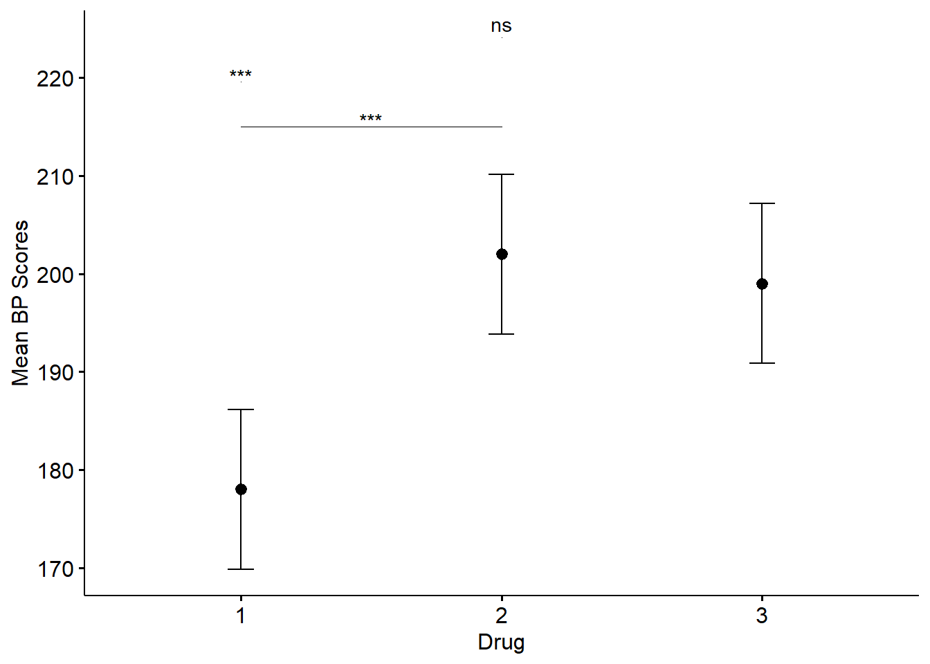
| Drug | Score | 1 | 2 | 24 | -4.300136 | 0.0002462 | 0.0002462 | *** |
| Drug | Score | 1 | 3 | 24 | -3.762619 | 0.0009578 | 0.0009578 | *** |
| Drug | Score | 2 | 3 | 24 | 0.537517 | 0.5958599 | 0.5958599 | ns |
# Print the estimated marginal means of Feedback
get_emmeans(pwc) %>% kableExtra::kable(., "html")
| Drug | emmean | se | df | conf.low | conf.high | method |
|---|---|---|---|---|---|---|
| 1 | 178 | 3.946518 | 24 | 169.8548 | 186.1452 | Emmeans test |
| 2 | 202 | 3.946518 | 24 | 193.8548 | 210.1452 | Emmeans test |
| 3 | 199 | 3.946518 | 24 | 190.8548 | 207.1452 | Emmeans test |
# Modify pwc to include x and y positions for plotting signficance markers
pwc <- pwc %>% add_xy_position(x = "Feedback", fun = "mean_ci")

# Generate an error plot uses ggpubr AND ggplot functions to layer the plot
ggerrorplot(get_emmeans(pwc),
       x = "Drug",
       y = "emmean",
       ylab = "Mean BP Scores") +
    geom_errorbar(aes(ymin = conf.low, ymax = conf.high),
                  width = 0.1) +
    stat_pvalue_manual(pwc, hide.ns = FALSE, tip.length = FALSE)

Figure 3: Means and confidence intervals for Drug collapsed across Feedback. *, p<0.05; **, p<0.01; ***, p<0.001; ns, not significant
# Generate an interaction plot
ggline(chapter_7_table_5,
       x = "Feedback",
       y = "Score",
       color = "Drug",
       add = "mean_se",
       palette = "jama",
       position = position_dodge(.2))
The two tests of marginal means will produce a couple of messages to remind us that the results could be misleading because of interactions. However, as we saw in the omnibus test, there was no significant interaction and can disregard the messages. The results of the emmeans_test() on Feedback indicate a significant effect and suggests that the participants undergoing biofeedback had lower bloodpressure scores than those without biofeedback. When examining the output of the results of the emmeans_test() on Drug, we see that the mean of Drug 1 is significantly lower than that of Drug 2 and Drug 3. However, the mean of Drug 2 is not significantly different than that of Drug 3.
Wrap up
The jmv and rstatix functions both produce the same results, as they should because they share many of the underlying statistical functions. The jmv package is a great place to start with statistical tests if you are beginning with R. One reason for this is because it simplifies some of the syntax, generates plots automatically, and it can automatically convert some of your numerical data to categorical. While it’s a lot easier to code a 2x3 ANOVA with jmv there are some advantages to using rstatix and ggpubr. One advantage is that the ggpubr functions are designed to take in arguments from rstatix that make plotting significance markers relatively straightforward. In addition, ggpubr plots can be used as a starting point to layer additional ggplot geometric elements like the geom_errorbar() in Figures 3 and 4.
References
Kassambara, Alboukadel. 2020a. Ggpubr: ’Ggplot2’ Based Publication Ready Plots. https://CRAN.R-project.org/package=ggpubr.
———. 2020b. Rstatix: Pipe-Friendly Framework for Basic Statistical Tests. https://CRAN.R-project.org/package=rstatix.
Maxwell, Scott, Harold Delaney, and Ken Kelley. 2020. AMCP: A Model Comparison Perspective. https://CRAN.R-project.org/package=AMCP.
Maxwell, Scott E, Harold D Delaney, and Ken Kelley. 2017. Designing Experiments and Analyzing Data: A Model Comparison Perspective. Routledge.
Selker, Ravi, Jonathon Love, and Damian Dropmann. 2020. Jmv: The ’Jamovi’ Analyses. https://CRAN.R-project.org/package=jmv.
Wickham, Hadley. 2019. Tidyverse: Easily Install and Load the ’Tidyverse’. https://CRAN.R-project.org/package=tidyverse.