One-way ANCOVA
In some situations, a researcher may wish to statistically control for a concomitant variable. A concomitant variable is one that “comes along” with other variables of interest. These variables are also known as covariates. The one-way analysis of covariance (ANCOVA) is one approach that is used to compare means of groups while accounting for a continuous covariate.
The data set
This guide uses data from Chapter 9, Table 7 in the AMCP package. In this hypothetical study, participants are randomly assigned to one of three conditions to examine the effectiveness of a treatment for depression. Participants received a selective serotonin reuptake inhibitor (SSRI) in condition 1, a placebo in condition 2, or were assigned to a wait list control in condition 3. Each participant was also assessed for depression with a pre- and post-treatment inventory. In this type of study, one might want to control for the pre-treatment levels of depression when comparing the three conditions in their post-treatment scores. As a result, pre-treatment depression scores can serve as covariates.
library(AMCP)

# Load data
data(chapter_9_table_7)

# Convert group to factor
chapter_9_table_7$Condition <- as.factor(chapter_9_table_7$Condition)

# Inspect Data
kableExtra::kable(head(chapter_9_table_7))
| Condition | Pre | Post |
|---|---|---|
| 1 | 18 | 12 |
| 1 | 16 | 0 |
| 1 | 16 | 10 |
| 1 | 15 | 9 |
| 1 | 14 | 0 |
| 1 | 20 | 11 |
Perform ANOVA Tests
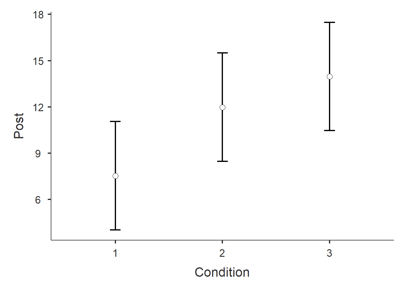
The following code chunk will perform a one-way ANCOVA predicting post-treatment depression scores by condition while considering pre-treatment depression scores as a covariate using Type III sums of squares. In addition, the call also asks to provide output for an effect size of partial eta squared for the omnibus test, to produce Bonferroni corrected post hoc tests to compare conditions, and post hoc test Cohen’s D effect size. Finally, a plot of means by condition with 95% confidence intervals will be generated.
library(jmv)

# ANCOVA in jmv
ancova(formula = Post ~ Pre + Condition,
       data = chapter_9_table_7,
       ss = "3",
       effectSize = 'partEta',
       postHoc = ~ Condition,
       postHocCorr = 'bonf',
       postHocES = "d",
       emMeans = ~ Condition,
       emmPlots = TRUE,
       emmTables = TRUE,
       emmPlotError = "ci",
       ciWidthEmm = 95)
##
##  ANCOVA
##
##  ANCOVA - Post
##  ───────────────────────────────────────────────────────────────────────────────────────────
##                 Sum of Squares    df    Mean Square    F            p            η²p
##  ───────────────────────────────────────────────────────────────────────────────────────────
##    Pre                313.3653     1      313.36526    10.772342    0.0029369    0.2929469
##    Condition          217.1495     2      108.57474     3.732399    0.0375843    0.2230642
##    Residuals          756.3347    26       29.08980
##  ───────────────────────────────────────────────────────────────────────────────────────────
##
##
##  POST HOC TESTS
##
##  Post Hoc Comparisons - Condition
##  ──────────────────────────────────────────────────────────────────────────────────────────────────────────────────────
##    Condition         Condition    Mean Difference    SE          df          t             p-bonferroni    Cohen's d
##  ──────────────────────────────────────────────────────────────────────────────────────────────────────────────────────
##    1            -    2                  -4.448279    2.415968    26.00000    -1.8411994       0.2310916    -0.8247488
##                 -    3                  -6.441874    2.413326    26.00000    -2.6692923       0.0387692    -1.1943782
##    2            -    3                  -1.993595    2.412766    26.00000    -0.8262695       1.0000000    -0.3696294
##  ──────────────────────────────────────────────────────────────────────────────────────────────────────────────────────
##    Note. Comparisons are based on estimated marginal means
##
##
##  ESTIMATED MARGINAL MEANS
##
##  CONDITION
##
##  Estimated Marginal Means - Condition
##  ───────────────────────────────────────────────────────────────
##    Condition    Mean         SE          Lower        Upper
##  ───────────────────────────────────────────────────────────────
##    1             7.536616    1.707096     4.027629    11.04560
##    2            11.984895    1.706832     8.476452    15.49334
##    3            13.978489    1.705586    10.472608    17.48437
##  ───────────────────────────────────────────────────────────────

Figure 1: Plot of post-treatment depression score means by Condition.
The following code chunk will produce the same ANCOVA output with the rstatix package. One slight difference here though is that we are going to save the output to an anova_test() object, then print the output with the get_anova_table() function. This approach will come in handy when generating the plot of means. In the anova_test() formula argument we enter the covariate first. This is primarily done to pull out the correct F ratio for plotting. In our example, we are setting the sums of squares type = 3 which means we will get the same output whether we use formula Post ~ Pre + Condition or formula = Post ~ Condition + Pre. However, if using Type II sums of squares enter the covariate first.
library(rstatix)
library(ggpubr)

# Evaluated ANCOVA test w rstatix
aocv.model <- anova_test(formula = Post ~  Pre + Condition,
                         data = chapter_9_table_7,
                         type = 3,
                         effect.size = "pes")

# Print ANOVA table
get_anova_table(aocv.model)
## ANOVA Table (type III tests)
##
##      Effect DFn DFd      F     p p<.05   pes
## 1       Pre   1  26 10.772 0.003     * 0.293
## 2 Condition   2  26  3.732 0.038     * 0.223
Post hoc tests
To conduct the post hoc tests, we will use the emmeans_test() function specifying the formula Post ~ Condition, setting covariate = Pre, and the Bonferroni correction with p.adjust.method = "bonferroni". In the following code chunk, we will also save the output to an object called pwc. The pwc object can be used with the get_emmeans() function to disply the estimated marginal means for each group after accounting for the covariate. Finally, we can print pwc to the console with the print() to display the results of the post hoc tests.
# Pairwise comparisons
pwc <- chapter_9_table_7 %>%
  emmeans_test(Post ~ Condition,
               covariate = Pre,
               p.adjust.method = "bonferroni")

# Print estimated marginal means
get_emmeans(pwc) %>% kableExtra::kable()
| Pre | Condition | emmean | se | df | conf.low | conf.high | method |
|---|---|---|---|---|---|---|---|
| 17.36667 | 1 | 7.536616 | 1.707096 | 26 | 4.027629 | 11.04560 | Emmeans test |
| 17.36667 | 2 | 11.984895 | 1.706832 | 26 | 8.476452 | 15.49334 | Emmeans test |
| 17.36667 | 3 | 13.978490 | 1.705586 | 26 | 10.472608 | 17.48437 | Emmeans test |
# Print post hoc tests
#print(pwc)
pwc %>% kableExtra::kable()
| term | .y. | group1 | group2 | df | statistic | p | p.adj | p.adj.signif |
|---|---|---|---|---|---|---|---|---|
| Pre*Condition | Post | 1 | 2 | 26 | -1.8411994 | 0.0770305 | 0.2310916 | ns |
| Pre*Condition | Post | 1 | 3 | 26 | -2.6692923 | 0.0129231 | 0.0387692 | * |
| Pre*Condition | Post | 2 | 3 | 26 | -0.8262695 | 0.4161696 | 1.0000000 | ns |
Effect sizes
The process to calculate the effect sizes of the post hoc comparisons is a little more drawn out in this case. First, we will need the MBESS package. Next we will need three pieces of information, group means, standard deviations, and sample sizes. We will want the estimated marginal means for this situation because these means have been adjusted to take into consideration the covariate. We can also calculate the standard deviations by multiplying the standard error of each group by the square root of the group sample size. Finally, we can enter those values into the smd() function which stands for the standardized mean difference. A nice feature of the smd() is that we can calculate a standardized mean difference as biased or unbiased. In practice, it is recommended to set Unbiased = TRUE with small samples.
library(MBESS)

# Get sample sizes. For these data, each group had 10 so n <- c(10, 10,10) would have worked,
# but the following code here will generalize to other datasets
n <- chapter_9_table_7 %>%
  group_by(Condition) %>%
  get_summary_stats() %>%
  filter(variable == "Post") %>%
  select(n)

# Need emmeans from pwc
emm <- get_emmeans(pwc) %>% select(emmean)

# Get standard deviations
std <- get_emmeans(pwc)$se * sqrt(n)

# Group 1 vs group 2
smd(Mean.1 = emm[1,],
    Mean.2 = emm[2,],
    s.1 = std[1,],
    s.2 = std[2,],
    n.1 = n[1,],
    n.2 = n[2,],
    Unbiased = FALSE)
##       emmean
## 1 -0.8240768
# Group 1 vs group 3
smd(Mean.1 = emm[1,],
    Mean.2 = emm[3,],
    s.1 = std[1,],
    s.2 = std[3,],
    n.1 = n[1,],
    n.2 = n[3,],
    Unbiased = FALSE)
##      emmean
## 1 -1.193841
# Group 2 vs group 3
smd(Mean.1 = emm[2,],
    Mean.2 = emm[3,],
    s.1 = std[2,],
    s.2 = std[3,],
    n.1 = n[2,],
    n.2 = n[3,],
    Unbiased = FALSE)
##       emmean
## 1 -0.3694917
Plot of means
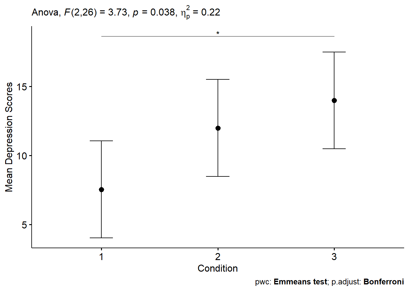
While the jmv approach is nice because we can get quite a bit of output (ANCOVA test, post hoc tests, and plots) from one function, the benefit of using rstatix is that we gain some additional features when it comes to plotting. The plot produced for this guide displays the estimated marginal means, confidence intervals, a significance marker, the results of the omnibust test, and includes a caption displaying the tests used to compare means and the multiple correction procedure.
# Add the x and y coordinates for plotting significance markers
pwc <- pwc %>% add_xy_position(x = "Condition",
                               fun = "mean_se")

# Generate an error plot with significance markers, label, and caption
ggerrorplot(get_emmeans(pwc),
            x = "Condition",
            y = "emmean",
            ylab = "Mean Depression Scores") +
  geom_errorbar(aes(ymin = conf.low, ymax = conf.high), width = 0.2) +
  stat_pvalue_manual(pwc, hide.ns = TRUE, tip.length = FALSE) +
  labs(subtitle = get_test_label(aocv.model, detailed = TRUE), caption = get_pwc_label(pwc))

Figure 2: Plot of post-treatment depression score means by Condition.
Interpretation
When examining the results of ANCOVA model, we notice that the pre-treatment scores significantly predicted post-treatment scores. Additionally, after removing the effect of the pre-treatment scores, the effect of Condition is signficant. By examining Figure 1 and the estimated marginal means seem lower for Condition 1. Post-hoc comparisons revealed a significant difference between Condition 1 and Condition 2, but not in any other pairwise test when correcting for multiple comparisons using the Bonferroni method.
Wrap up
So far, we have seen that the jmv package is well suited for conducting between-subjects ANOVA and ANCOVA. However, we can also appreciate that the rstatix and ggpubr packages work well together for visualizing data. For this guide, the combination of the emmeans_test(), add_xy_position(), and stat_pvalue_manual() functions make plotting means and the statistical significance between them and added feature that can come in handy for preparing publication ready figures.
Suggested reading
Miller, G. A., and J. P. Chapman. 2001. “Misunderstanding Analysis of Covariance.” Journal Article. J Abnorm Psychol 110 (1): 40–48. https://doi.org/10.1037//0021-843x.110.1.40.
References
Kassambara, Alboukadel. 2020a. Ggpubr: ’Ggplot2’ Based Publication Ready Plots. https://CRAN.R-project.org/package=ggpubr.
———. 2020b. Rstatix: Pipe-Friendly Framework for Basic Statistical Tests. https://CRAN.R-project.org/package=rstatix.
Maxwell, Scott, Harold Delaney, and Ken Kelley. 2020. AMCP: A Model Comparison Perspective. https://CRAN.R-project.org/package=AMCP.
Maxwell, Scott E, Harold D Delaney, and Ken Kelley. 2017. Designing Experiments and Analyzing Data: A Model Comparison Perspective. Routledge.
Selker, Ravi, Jonathon Love, and Damian Dropmann. 2020. Jmv: The ’Jamovi’ Analyses. https://CRAN.R-project.org/package=jmv.
Wickham, Hadley. 2019. Tidyverse: Easily Install and Load the ’Tidyverse’. https://CRAN.R-project.org/package=tidyverse.